Chapter 6 Hypothesis Tests

6.1 Introduction

A hypothesis test is a statistical method used to make inferences about a population based on sample data. It involves formulating a null hypothesis and an alternative hypothesis, calculating a test statistic, and determining the likelihood of observing the data under the null hypothesis. Each of these terms will be explained in more detail below.

Definition 6.1 An inferential procedure to determine whether there is sufficient evidence to suggest a condition for a population parameter using statistics from a sample.

The main goal of hypothesis testing is to assess the strength of evidence against a null hypothesis, which is a statement of no effect or no difference. The alternative hypothesis represents the research hypothesis or the condition we are interested in testing.

One of the steps in hypothesis testing is to calculate a p-value, which quantifies the evidence against the null hypothesis. The p-value is the probability of observing a test statistic at least as extreme as the one calculated from the sample data, assuming that the null hypothesis is true.

Definition 6.2 The p-value of a hypothesis test is the probability of observing a test statistic at least as extreme as the one calculated in step 3, assuming that the null hypothesis is true by pure chance alone.

The procedure to conduct any hypothesis often follows a standard sequence of steps.

Steps

[Reorder and start with checking assumptions first?]

1. Decide on a level of significance (\(\alpha\)).

2. State the null hypothesis (\(H_0\)) and the alternative hypothesis (\(H_a\)).

3. Calculate the appropriate test statistic.

4. Use the test statistic and a reference distribution to calculate a p-value.

5. Compare p-value to \(\alpha\) to make a conclusion.

We will now examine each of the steps above in more detail.

Step 1: Decide on a Level of Significance (\(\alpha\))

This is a threshold for decision making which the study or researcher is willing to implement. Depends on tolerance for consequences of errors, sample size, nature of the study, and variability.

Some common Common values are \(\alpha = 0.10\), \(\alpha = 0.05\), \(\alpha = 0.01\).

Step 2: State the Null Hypothesis and the Alternative Hypothesis

We will use the following notation for describing the null and alternative hypotheses:

\(\Theta\) : Parameter of interest. \(\Theta_0\) : Numerical value hypothesized under the null hypothesis.

Remark. Note that \(\Theta\) can represent a combination of parameters, such as \(\Theta = \Theta_1 - \Theta_2\) or \(\Theta = \Theta_1 / \Theta_2\).

A hypothesis test is a comparison between two mutually exclusive hypotheses which are:

Null hypothesis \((H_0)\)	:	Represents the current belief or the conservative belief or the status quo. It is a statement of no effect or no difference.
Alternative hypothesis \((H_a)\)	:	Represents the research hypothesis, or what you are requested to test or trying to prove.

Our choices for the null and alternative hypothesis are:

\(H_0: \Theta = \Theta_0\)	vs.	\(H_a: \Theta > \Theta_0\)
\(H_0: \Theta = \Theta_0\)	vs.	\(H_a: \Theta < \Theta_0\)
\(H_0: \Theta = \Theta_0\)	vs.	\(H_a: \Theta \neq \Theta_0\)

Remark. The first two hypothesis tests above are referred to as one-sided or one-tailed tests. and the third hypothesis test is referred to as a two-sided or two-tailed test.

Remark. The one-sided hypothesis test \[\begin{array}{lcl} H_0: \Theta = \Theta_0 & \quad & H_a: \Theta > \Theta_0\\ \end{array}\] is equivalent to \[\begin{array}{lcl} H_0: \Theta \leq \Theta_0 & \quad & H_a: \Theta > \Theta_0\\ \end{array}\]

and the other one-sided hypothesis test

\[\begin{array}{lcl} H_0: \Theta = \Theta_0 & \quad & H_a: \Theta < \Theta_0\\ \end{array}\] is equivalent to \[\begin{array}{lcl} H_0: \Theta \geq \Theta_0 & \quad & H_a: \Theta < \Theta_0\\ \end{array}\]

Step 3: Calculate an appropriate test statistic

Depends on the hypothesis test conducted and the information available.

Definition 6.3 \[\text{test statistic} = \frac{\text{(a statistic)} - \text{(hypothesized value of parameters under } H_0 \text{)}}{\text{standard error of statistic}}\]

The test statistic follows a reference distribution. Common distributions which thetest statistic follows are the standard normal distrubution, \(t\)-distribution, \(F\)-distribution and \(\chi^2\)-distribution.

Step 4: Calculate the p-value

We use the test statistic, reference distribution, and refer back to \(H_a\).

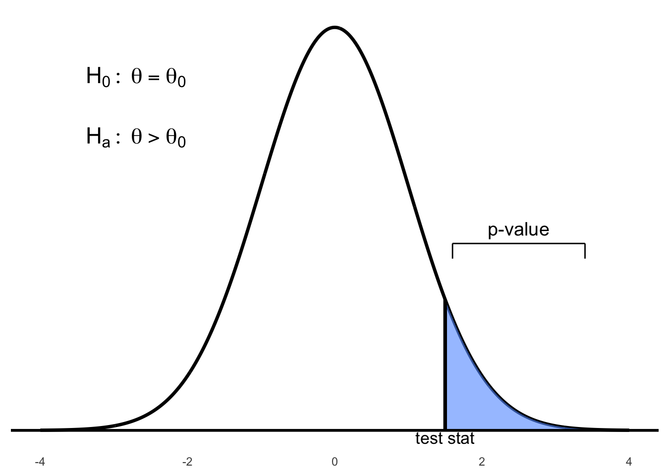
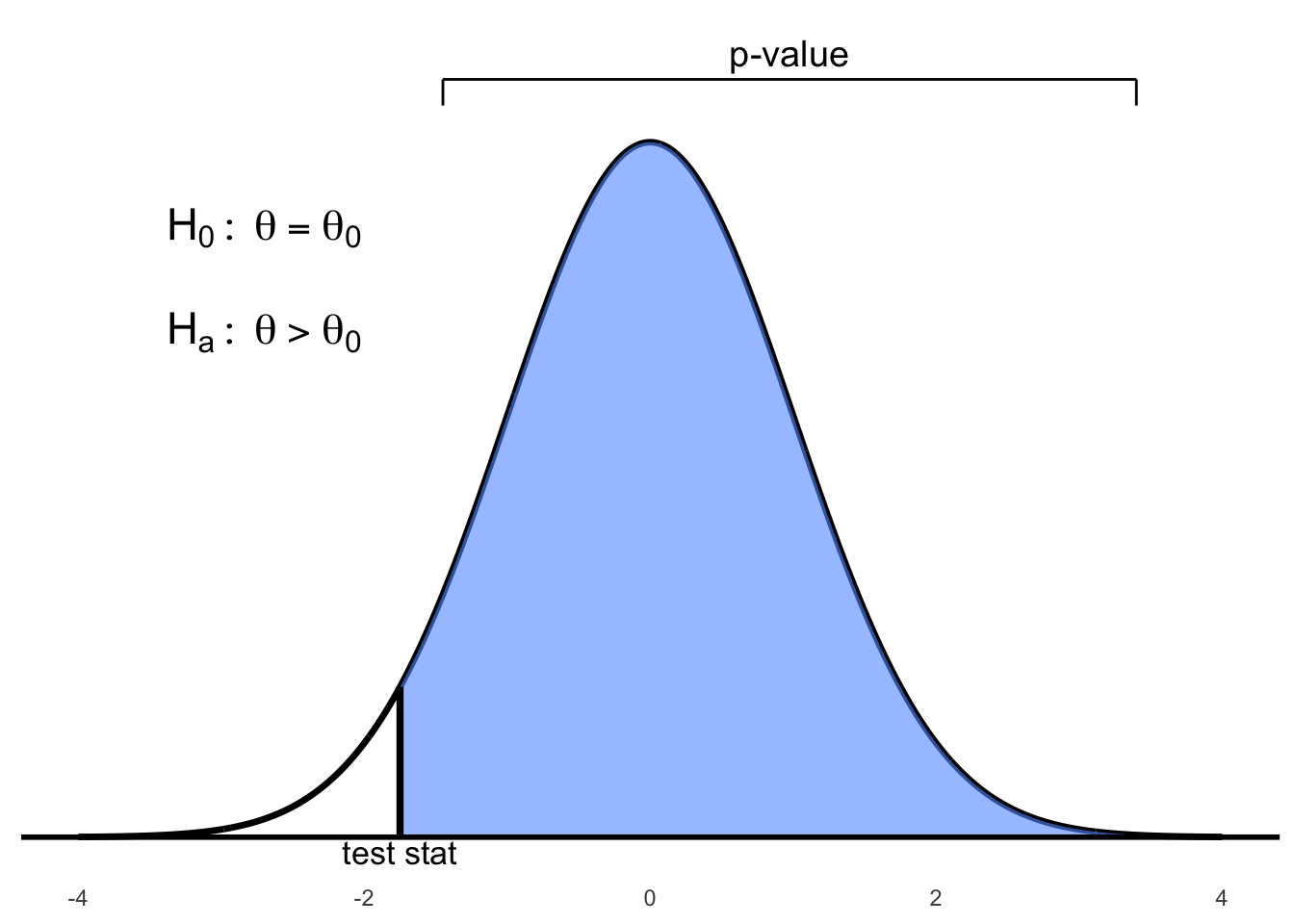
Figure 6.1: Right-tailed test: p-value is the area to the right of the test statistic

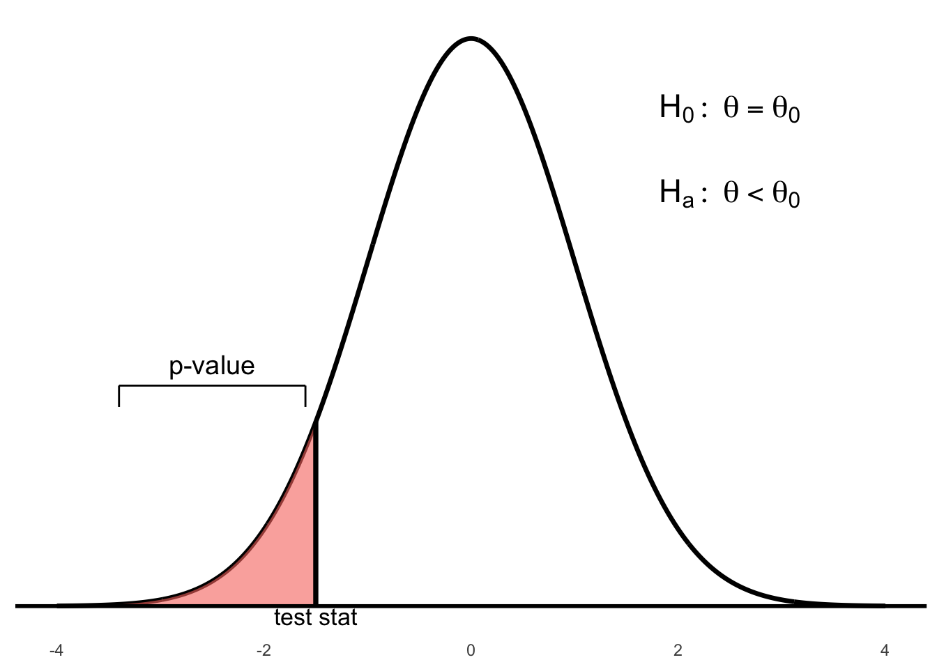
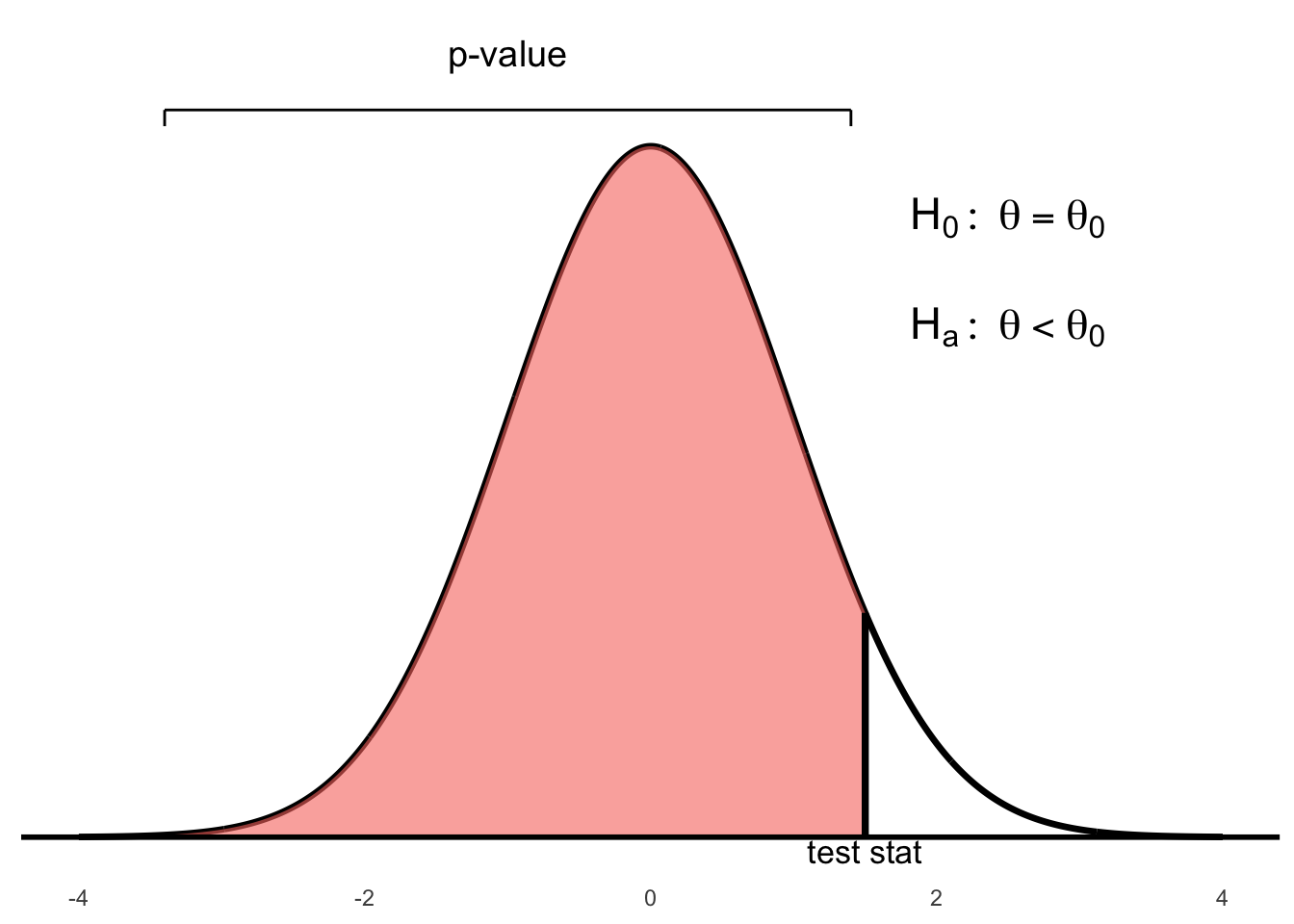
Figure 6.2: Left-tailed test: p-value is the area to the left of the test statistic

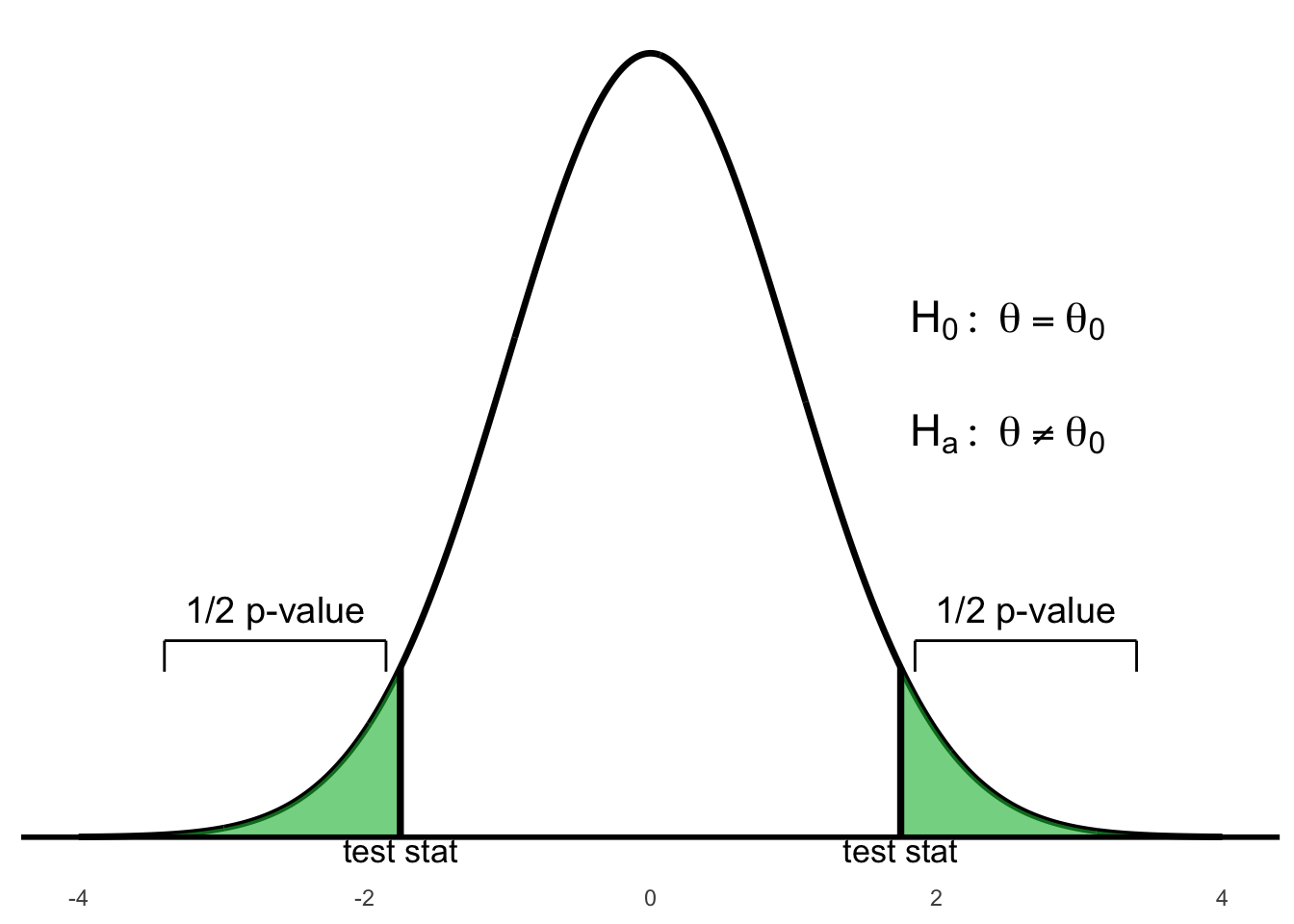
Figure 6.3: Two-tailed test: p-value is the total area in both tails beyond ±test statistic

Step 5: Compare p-value to level of significance \(\alpha\) and make a conclusion

• If the p-value \(< \alpha\), we say there is sufficient evidence against \(H_0\) and the hypothesis test rejects \(H_0\) in favor of \(H_a\).

• If the p-value \(> \alpha\), thenwe say there is insufficient evidence against \(H_0\) and we do not reject \(H_0\) (in this situation we can also say fail to reject \(H_0\)).

About the p-value of the test statistics

• The p-value is a conditional probability.

• It is not the probability that \(H_0\) (null hypothesis: current belief) is true.

• It is: P(observed statistic value — \(H_0\)). Given \(H_0\) (the null hypothesis), because \(H_0\) gives the parameter values that we need to find required probability.

• The p-value serves as a measure of the strength of the evidence against the null hypothesis (but it should not serve as a hard and fast rule for decision).

• If the p-value = 0.03 (for example) all we can say is that there is 3% chance of observing the statistic value we actually observed (or one even more inconsistent with the null value).

• The p-value is the chance (the proportion) of getting a, for instance, \(\hat{p}\) as far as or further from \(H_0\) than the value observed.

• The p-value is the probability of getting at least something (e.g., sample proportion \(\hat{p}\)) more extreme (e.g., unusual, unlikely, or rare) than what we have already found (our observed value of \(\hat{p}\)) that provide even stronger evidence against \(H_0\).

• The more extreme the z-score (large in absolute values) are the ones that denote farther departure of the observed value (e.g., our \(\hat{p}\)) from the parameter value (\(p_0\)) in \(H_0\).

• In the one-sided test, e.g., \(H_a : p > p_0\), p-value is one-tailed probability. This is the probability that sample proportion \(\hat{p}\) falls at least as far from \(p_0\) in one direction as the observed value of \(\hat{p}\).

• In the two-sided test, e.g., \(H_a : p \ne p_0\), p-value is two-tailed probability. This is the probability that sample proportion \(\hat{p}\) falls at least as far from \(p_0\) in either direction as the observed value of \(\hat{p}\).

The probability, computed assuming that \(H_0\) is true, that the test statistic would take a value as extreme or more extreme than that actually observed is called the P-value of the test. The smaller the P-value, the stronger the evidence against \(H_0\) provided by the data.

Small P-values are evidence against \(H_0\), because they say that the observed result is unlikely to occur when \(H_0\) is true. Large P-values fail to give evidence against \(H_0\).

The P-value Scale

• If P-value \(<\) 0.001, we have very strong evidence against \(H_0\).

• If 0.001 \(\leq\) P-value \(<\) 0.01, we have strong evidence against \(H_0\).

• If 0.01 \(\leq\) P-value \(<\) 0.05, we have evidence against \(H_0\).

• If 0.05 \(\leq\) P-value \(<\) 0.075, we have some evidence against \(H_0\).

• If 0.075 \(\leq\) P-value \(<\) 0.10, we have slight evidence against \(H_0\).

Use p-value Method to Make a Decision (Reject or Fail to Reject \(H_0\))

But how small is small p-value?
We would need to choose an \(\alpha\)-level (significance-level): a number such that if:

• \(P\text{–value} \leq \alpha\)-level, we reject \(H_0\); We can conclude \(H_a\) (we have evidence to support our claim). Often we phrase as a statistically significant result at that specified \(\alpha\)-level.

• \(P\text{–value} > \alpha\)-level, we fail to reject \(H_0\); We cannot conclude \(H_a\) (we have not enough evidence to support our claim; thus, \(H_0\) is plausible - We do not accept \(H_0\)). Often we phrase as the result is not statistically significant at that specified \(\alpha\)-level.

• The default \(\alpha\)-level (significance-level) is typically \(\alpha = 0.05\) (but it can be different based on the context of the study - it is usually not higher than 0.10).

The p-value in the previous example was extremely small (less than 0.0001). That is a strong evidence to suggest that more than 5% of children have genetic abnormalities. However, it does not say that the percentage of sampled children with genetic abnormalities was “a lot more than 5%”. That is, the p-value by itself says nothing about how much greater the percentage might be. The confidence interval provides that information.
To assess the difference in practical terms, we should also construct a confidence interval:

\[0.1198 \pm (1.96 \times 0.0166)\] \[0.1198 \pm 0.0324\] \[(0.0874,\ 0.1522)\]

Interpretation: We are 95% Confident that the true percentage of children with genetic abnormalities is between 8.74% and 15.22%.
95% CI for \(p\): (9.1%, 15.6%) – We are 95% confident that the true percentage of all children that have genetic abnormalities is between approximately 9.1% and 15.6%. Since both values of this CI are more than the hypothesized value of \(p = 0.05\) (5%), we can further infer that this true percentage is more than 5%.
Do environmental chemicals cause congenital abnormalities?

We do not know that environmental chemicals cause genetic abnormalities. We merely have evidence that suggests that a greater percentage of children are diagnosed with genetic abnormalities now, compared to the 1980s.

More About P-values

• Big p-values just mean that what we have observed is not surprising. It means that the results are in line with our assumption that the null hypothesis models the world, so we have no reason to reject it.

• A big p-value does not prove that the null hypothesis is true.

• When we see a big p-value, all we can say is: we cannot reject \(H_0\) (we fail to reject \(H_0\)) – we cannot conclude \(H_a\) (We have no evidence to support \(H_a\)).

6.2 One Sample Hypothesis Tests

6.2.1 On a Population Mean

6.2.1.1 When \(\sigma\) is Known

To test \(H_0 : \mu = \mu_0\), in the situation where the population standard deviation \(\sigma\) is known, our options for the null and alternative hypotheses are:

• \(H_0: \mu = \mu_0\) vs. \(H_a: \mu > \mu_0\)

• \(H_0: \mu = \mu_0\) vs. \(H_a: \mu < \mu_0\)

• \(H_0: \mu = \mu_0\) vs. \(H_a: \mu \neq \mu_0\)

We calculate the \(z\)-statistic:

\[z^{*} = \frac{\bar{x} - \mu_0}{\sigma / \sqrt{n}} \sim N(0,1)\]

The reference distribution is the standard normal distribution.

In terms of a variable \(Z\) having the standard normal distribution, the p-value for a test of \(H_0\) against:

• \(H_a: \mu > \mu_0\) is \(P(Z > z^{*})\)

• \(H_a: \mu < \mu_0\) is \(P(Z < z^{*})\)

• \(H_a: \mu \ne \mu_0\) is \(2P(Z > |z^{*}|)\)

Example 6.1 Deer are a common sight on the UTM campus. Suppose an ecologist is interested in the average mass of adult white-tailed does (female deer) around the Mississauga campus to determine whether they are healthy for the upcoming winter. The ecologist captures a sample of 36 adult females around the UTM and measures the average mass of this sample to be 42.53 kg.

From previous studies conducted in the area, the average mass of healthy does was reported to be 45 kg. Conduct a hypothesis test at the 5% significance level to determine whether the mass of does around UTM has decreased. Assume the standard deviation is known to be 5.25 kg.

1. Level of significance. \(\alpha = 0.05\)

2. State the null and alternative hypotheses. \[H_0: \mu = 45 \qquad H_a: \mu < 45\]

3. Calculate appropriate test statistic.

Given: \[n = 36, \quad \bar{x} = 42.53, \quad \sigma = 5.25\]

Since \(\sigma\) is known, the test statistic is: \[z^* = \frac{\bar{x} - \mu_0}{\sigma / \sqrt{n}} = \frac{42.53 - 45}{5.25/\sqrt{36}} = -2.82\]

Reference distribution: standard normal

4. Calculate p-value

\[\text{p-value} = P(Z < -2.82) \approx 0.0024\]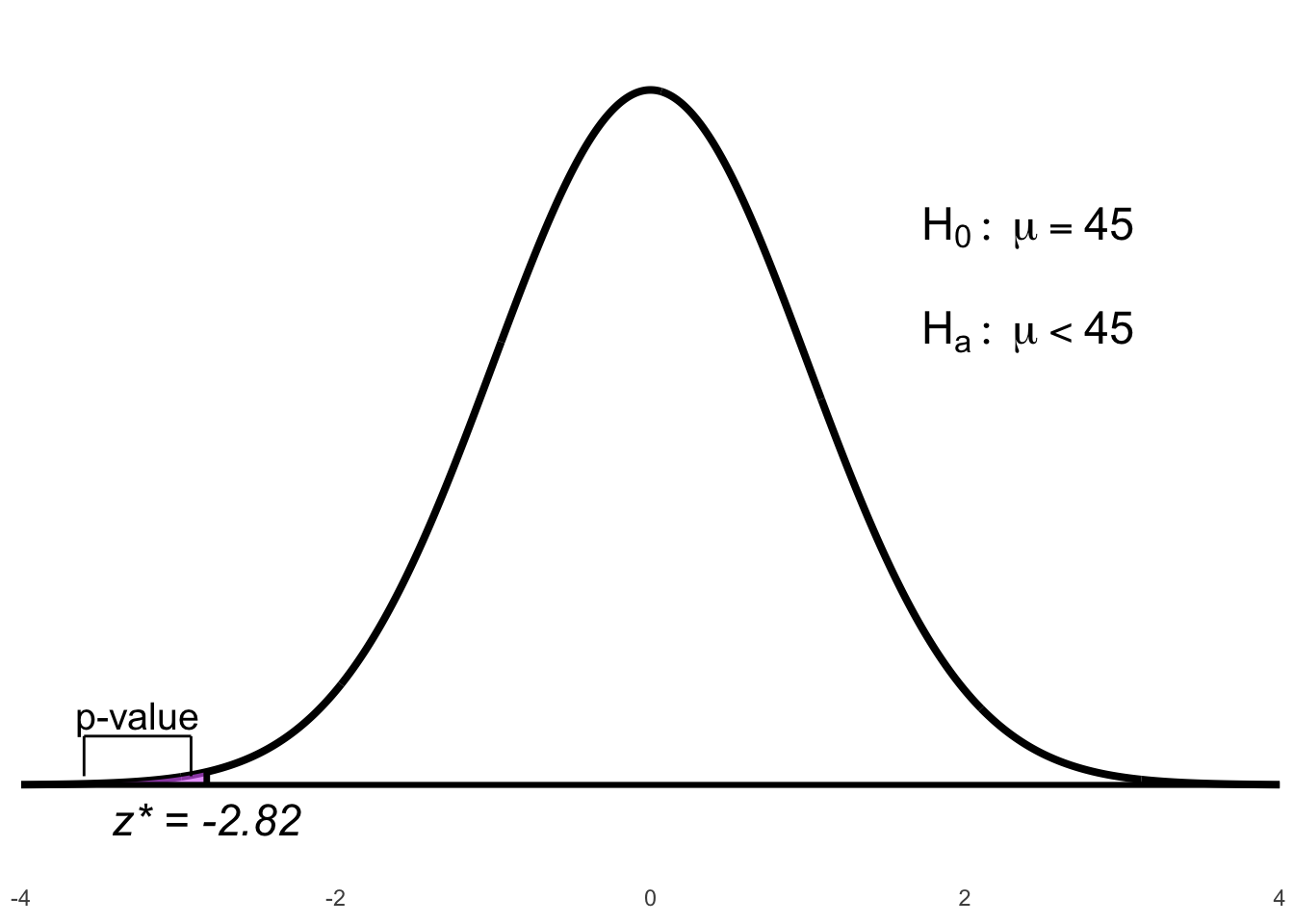

Figure 6.4: Left-tailed p-value for the test statistic \(z^* = -2.82\)

5. Compare p-value with level of significance \(\alpha\) and make a conclusion:

\[0.0024 < 0.05 \Rightarrow \text{p-value} < \alpha\]

There is sufficient evidence at the 5% level of significance to reject the null that does this winter weigh the same as in the past and to conclude the alternative that does this winter weigh less than 45 kg.

R code:

    # Find test stat
    z_test_stat = (42.53 - 45) / (5.25 / sqrt(36))
    z_test_stat
    [1] -2.822857

    # Find the p-value
    # Since the alternative is Ha : mu < 45
    p-value = pnorm(z_test_stat)
    [1] 0.00237989

Note: The pnorm() function in R, by default, returns the cumulative probability (area) to the left of the given value.

R code: Using BSDA package

    # Using the BSDA library. install BSDA if it is not already installed.
    # install.packages("BSDA")
    > library(BSDA)
    > # Conduct the z-test with the zsum.test function
    > zsum.test(mean.x = 42.53, sigma.x = 5.24, n.x = 36, mu = 45, alternative = "less")

            One-sample z-Test

    data:  Summarized x
    z = -2.8282, p-value = 0.00234
    alternative hypothesis: true mean is less than 45
    95 percent confidence interval:
     NA 43.96651
    sample estimates:
    mean of x 
        42.53 

Interpretation:

There is sufficient evidence at the 5% level of significance to reject the null hypothesis. We conclude that the average mass of does this winter is significantly less than 45 kg.

Example 6.2 Diet colas use artificial sweeteners to avoid sugar. These sweeteners gradually lose their sweetness over time. Manufacturers therefore test new colas for loss of sweetness before marketing them. Trained tasters sip the cola along with drinks of standard sweetness and score the cola on a “sweetness score” of 1 to 10. The cola is then stored for a month at high temperature to imitate the effect of four months’ storage at room temperature. Each taster scores the cola again after storage. This is a matched pairs experiment. Our data are the differences (score before storage minus score after storage) in the tasters’ scores. The bigger these differences, the bigger the loss of sweetness.

Suppose we know that for any cola, the sweetness loss scores vary from taster to taster according to a Normal distribution with standard deviation \(\sigma = 1\). The mean \(\mu\) for all tasters measures loss of sweetness.

The following are the sweetness losses for a new cola as measured by 10 trained tasters:

\[2.0, 0.4, 0.7, 2.0, -0.4, 2.2, -1.3, 1.2, 1.1, 2.3\]

Are these data good evidence that the cola lost sweetness in storage?
Solution
\(\mu\) = mean sweetness loss for the population of all tasters.
Step 1: State hypotheses. \[\begin{aligned} H_0 &: \mu = 0 \\ H_a &: \mu > 0 \end{aligned}\] Step 2: Test statistic: \(z_\star = \dfrac{\bar{x} - \mu_0}{\sigma / \sqrt{n}} = \dfrac{1.02 - 0}{1 / \sqrt{10}} = 3.23\)
Step 3: P-value. \(P(Z > z_\star) = P(Z > 3.23) = 0.0006\)
Step 4: Conclusion. We would rarely observe a mean as large as 1.02 if \(H_0\) were true. The small p-value provides strong evidence against \(H_0\), supporting \(H_a: \mu > 0\). That is, the mean sweetness loss is likely positive.

R code (Simulation)

    # n = sample size;
    n<-10;
    mu.zero<-0;
    sigma<-1;
    sigma.xbar<-sigma/sqrt(n);

    # x bar = sample mean with 10 obs;
    x.bar<-rnorm(1,mean=mu.zero,sd=sigma.xbar);
    x.bar;

    ## [1] 0.3265859

    # z.star = test statistic;
    z.star<-(x.bar-mu.zero)/sigma.xbar;
    z.star;

    ## [1] 1.032755

R code (10,000 Simulations)

    n <- 10;
    mu.zero <- 0;
    sigma <- 1;
    sigma.xbar <- sigma / sqrt(n);
    # x bar = sample mean with 10 obs;
    # m = number of simulations;
    m <- 10000;
    x.bar <- rnorm(m, mean = mu.zero, sd = sigma.xbar);

    # z.star = test statistic;
    z.star <- (x.bar - mu.zero) / sigma.xbar;
    hist(z.star, xlab = "differences", col = "blue");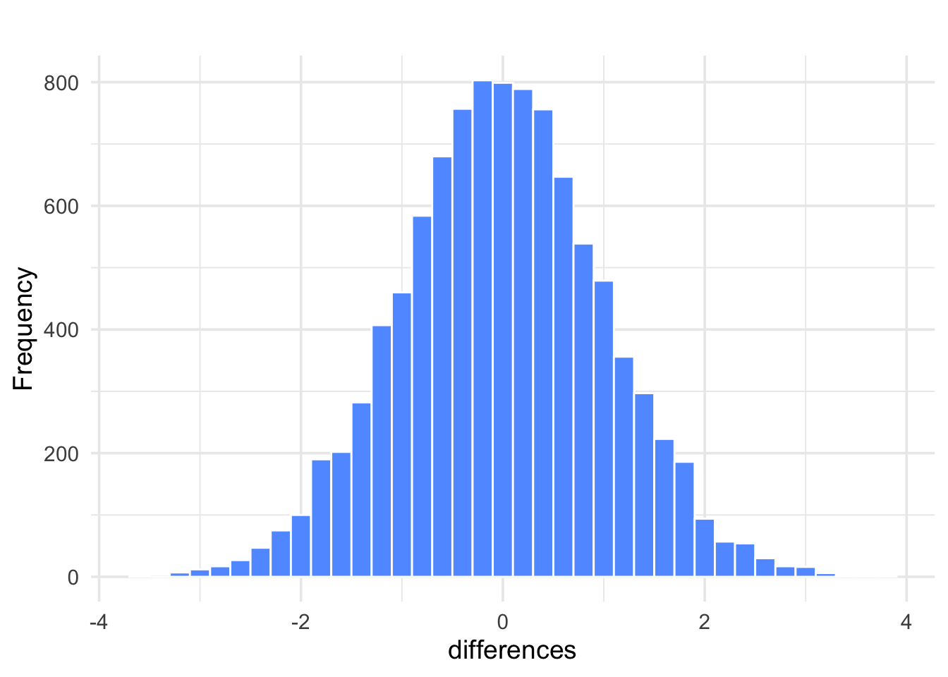

Figure 6.5: Histogram of \(z^\star\) values from 10,000 simulations under \(H_0\)

R code (Empirical p-value)

    ## P-value

    p_value <- length(z.star[z.star > 3.23]) / m;

    p_value

    ## [1] 8e-04

Example 6.3 The National Center for Health Statistics reports that the systolic blood pressure for males 35 to 44 years of age has mean 128 and standard deviation 15.

The medical director of a large company looks at the medical records of 72 executives in this age group and finds that the mean systolic blood pressure in this sample is \(\bar{x} = 126.07\). Is this evidence that the company’s executives have a different mean blood pressure from the general population?

Suppose we know that executives’ blood pressures follow a Normal distribution with standard deviation \(\sigma = 15\).

Solution: Let \(\mu\) be the mean systolic blood pressure of the executive population.

1. State hypotheses:
   \[\begin{aligned} H_0 &: \mu = 128 \\ H_a &: \mu \ne 128 \end{aligned}\]

2. Test statistic:
   \[z^{*} = \frac{\bar{x} - \mu_0}{\sigma / \sqrt{n}} = \frac{126.07 - 128}{15 / \sqrt{72}} = -1.09\]

3. P-value:
   \[2P(Z > |z^{*}|) = 2P(Z > 1.09) = 2(1 - 0.8621) = 0.2758\]

4. Conclusion:
   More than 27% of the time, a simple random sample of size 72 from the general male population would have a mean blood pressure at least as far from 128 as that of the executive sample. The observed \(\bar{x} = 126.07\) is therefore not good evidence that executives differ from other men.

Example 6.4 Consider the following hypothesis test:

\[\begin{aligned} H_0 &: \mu = 20 \\ H_a &: \mu < 20 \end{aligned}\]

A sample of 50 provided a sample mean of 19.4. The population standard deviation is 2.

1. Compute the value of the test statistic.

2. What is the p-value?

3. Using \(\alpha = 0.05\), what is your conclusion?

Solution:

1. Test statistic: \[z^{*} = \frac{\bar{x} - \mu_0}{\sigma / \sqrt{n}} = \frac{19.4 - 20}{2 / \sqrt{50}} = -2.1213\]

2. P-value: \[P(Z < z^{*}) = P(Z < -2.1213) = 0.0169\]

3. Conclusion:
   Since the p-value \(= 0.0169 < \alpha = 0.05\), we reject \(H_0 : \mu = 20\). We conclude that \(\mu < 20\).

Example 6.5 Consider the following hypothesis test:

\[\begin{aligned} H_0 &: \mu = 25 \\ H_a &: \mu > 25 \end{aligned}\]

A sample of 40 provided a sample mean of 26.4. The population standard deviation is 6.

1. Compute the value of the test statistic.

2. What is the p-value?

3. Using \(\alpha = 0.01\), what is your conclusion?

Solution:

1. Test statistic: \[z^{*} = \frac{\bar{x} - \mu_0}{\sigma / \sqrt{n}} = \frac{26.4 - 25}{6 / \sqrt{40}} = 1.4757\]

2. P-value: \[P(Z > z^{*}) = P(Z > 1.4757) = 0.0700\]

3. Conclusion:
   Since the p-value \(= 0.0700 > \alpha = 0.01\), we cannot reject \(H_0 : \mu = 25\).
   We conclude that we don’t have enough evidence to claim that \(\mu > 25\).

Example 6.6 Consider the following hypothesis test:

\[\begin{aligned} H_0 &: \mu = 15 \\ H_a &: \mu \ne 15 \end{aligned}\]

A sample of 50 provided a sample mean of 14.15. The population standard deviation is 3.

1. Compute the value of the test statistic.

2. What is the p-value?

3. Using \(\alpha = 0.05\), what is your conclusion?

Solution:

1. Test statistic: \[z^{*} = \frac{\bar{x} - \mu_0}{\sigma / \sqrt{n}} = \frac{14.15 - 15}{3 / \sqrt{50}} = -2.0034\]

2. P-value: \[2P(Z > |z^{*}|) = 2P(Z > |{-2.0034}|) = 2P(Z > 2.0034) = 0.0451\]

3. Conclusion:
   Since P-value \(= 0.0451 < \alpha = 0.05\), we reject \(H_0 : \mu = 15\).
   We conclude that \(\mu \ne 15\).

Confidence Interval Interpretation:

The 95% confidence interval for \(\mu\) is: \[\bar{x} \pm z^{*} \left( \frac{\sigma}{\sqrt{n}} \right)\] \[14.15 \pm 1.96 \left( \frac{3}{\sqrt{50}} \right) = (13.3184,\ 14.9815)\]

Since the hypothesized value \(\mu_0 = 15\) falls outside this interval, we again reject \(H_0 : \mu = 15\).

6.2.1.2 When \(\sigma\) is Not Known

To test \(H_0 : \mu = \mu_0\), in the situation where the population standard deviation \(\sigma\) is not known, our options for the null and alternative hypotheses are:

• \(H_0: \mu = \mu_0\) vs. \(H_a: \mu > \mu_0\)

• \(H_0: \mu = \mu_0\) vs. \(H_a: \mu < \mu_0\)

• \(H_0: \mu = \mu_0\) vs. \(H_a: \mu \neq \mu_0\)

We calculate the \(t\)-statistic:

\[t^{*} = \frac{\bar{x} - \mu_0}{s / \sqrt{n}} \sim t_{n-1}\]

In terms of a variable \(T\) which follows a \(t\)-distribution at \(n-1\) degrees of freedom, the p-value for a test of \(H_0\) against:

• \(H_a: \mu > \mu_0\) is \(P(T > t^{*})\)

• \(H_a: \mu < \mu_0\) is \(P(T < t^{*})\)

• \(H_a: \mu \ne \mu_0\) is \(2P(T > |t^{*}|)\)

Example 6.7 Researchers studied the physiological effects of laughter. They measured heart rates (in beats per minute) of \(n = 25\) subjects (ages 18–34) while they laughed. They obtained: \[\bar{x} = 73.5, \quad s = 6, \quad \alpha = 0.05\] It is well known that the resting heart rate is 71 bpm. Is there evidence that the mean heart rate during laughter exceeds 71 bpm?

Step 1: State the hypotheses. \[\begin{aligned} H_0 &: \mu = 71 \\ H_a &: \mu > 71 \end{aligned}\]

Step 2: Check assumptions.

• The sample is an independent random sample of individuals aged 18–34.

• The population of heart rates during laughter is normally distributed.

Step 3: Compute the test statistic.

Since \(\sigma\) is unknown, we use the \(t\) statistic: \[t^\ast = \frac{\bar{x} - \mu_0}{s / \sqrt{n}} = \frac{73.5 - 71}{6 / \sqrt{25}} = 2.083\]

Reference distribution: \(t\) distribution with \(n - 1 = 25 - 1 = 24\) degrees of freedom.

Step 4: Determine the p-value.

Using the \(t\) distribution with 24 df: \[0.01 < \text{p-value} < 0.025\]

Step 5: Make a conclusion.

Since \(\text{p-value} < \alpha = 0.05\), we reject \(H_0\).

There is sufficient evidence at the 5% level of significance to reject the null that the mean is 71 bpm in favor of the alternative that the mean is greater than 71 bpm for people who are laughing.

Example 6.8 A researcher is asked to test the hypothesis that the average price of a 2-star (CAA rating) motel room has decreased since last year. Last year, a study showed that the prices were Normally distributed with a mean of $89.50.

A random sample of twelve 2-star motels produced the following room prices:

\[\text{\$85.00, 92.50, 87.50, 89.90, 90.00, 82.50, 87.50, 90.00, 85.00, 89.00, 91.50, 87.50}\]

At the 5% level of significance, can we conclude that the mean price has decreased?

Solution:

Let \(\mu\) be the true average price of a 2-star motel room.

1. State hypotheses. \[\begin{aligned} H_0 &: \mu = 89.5 \\ H_a &: \mu < 89.5 \end{aligned}\]

2. Compute test statistic. \[t^\ast = \frac{\bar{x} - \mu_0}{s / \sqrt{n}} = \frac{88.1583 - 89.5}{2.9203 / \sqrt{12}} = -1.5915\]

3. Find the p-value.
   With \(df = 11\), the p-value (from the \(t\)-distribution table) is between 0.05 and 0.10.

4. Conclusion.
   Since the p-value \(> 0.05\), we fail to reject \(H_0\).
   There is not sufficient evidence to conclude that the average price of 2-star motels has decreased this year.

R code (One Sample t-test)

    # Step 1. Entering data;
    prices=c(85.00, 92.50, 87.50, 89.90, 90.00, 82.50,
             87.50, 90.00, 85.00, 89.00, 91.50, 87.50);

    # Step 2. Hypothesis test;
    t.test(prices, alternative="less", mu=89.5);

R output

    ## 
    ##  One Sample t-test
    ## 
    ## data:  prices
    ## t = -1.5915, df = 11, p-value = 0.0699
    ## alternative hypothesis: true mean is less than 89.5
    ## 95 percent confidence interval:
    ##  -Inf 89.67229
    ## sample estimates:
    ## mean of x 
    ##  88.15833 

Draw an SRS of size \(n\) from a large population having unknown mean \(\mu\).

To test the hypothesis \(H_0 : \mu = \mu_0\), compute the one-sample \(t\) statistic \[t^\ast = \frac{\bar{x} - \mu_0}{s / \sqrt{n}}\]

In terms of a variable \(T\) having the \(t_{n - 1}\) distribution, the p-value for a test of \(H_0\) against

\[\begin{aligned} H_a : \mu > \mu_0 &\quad \text{is} \quad P(T \ge t^\ast) \\ H_a : \mu < \mu_0 &\quad \text{is} \quad P(T \le t^\ast) \\ H_a : \mu \ne \mu_0 &\quad \text{is} \quad 2P(T \ge |t^\ast|) \end{aligned}\]

These p-values are exact if the population distribution is Normal and are approximately correct for large \(n\) in other cases.

Example 6.9 We are conducting a two-sided one-sample \(t\)-test for the hypotheses: \[\begin{aligned} H_0 &: \mu = 64 \\ H_a &: \mu \ne 64 \end{aligned}\]

based on a sample of \(n = 15\) observations, with test statistic \(t^* = 2.12\).

a) Degrees of freedom:

\[df = n - 1 = 15 - 1 = 14\]

b) Critical values and p-value bounds:

From the \(t\)-distribution table for \(df = 14\):

• \(t = 1.761\) corresponds to a two-tailed probability of 0.10

• \(t = 2.145\) corresponds to a two-tailed probability of 0.05

Since \(t^* = 2.12\) falls between these values, the two-sided p-value satisfies: \[0.05 < \text{p-value} < 0.10\]

c) Significance:

• At the 10% level: Yes, since the p-value \(< 0.10\)

• At the 5% level: No, since the p-value \(> 0.05\)

d) Exact two-sided p-value using R:

    # Compute exact two-sided p-value for t* = 2.12 with df = 14
    2 * (1 - pt(2.12, df = 14))

    ## [1] 0.05235683

Thus, the exact two-sided p-value is approximately 0.0524, confirming the bracketing result.

6.2.2 On a Population Proportion

To test \(H_0 : p = p_0\), our options for the null and alternative hypotheses are:

• \(H_0: p = p_0\) vs. \(H_a: p > p_0\)

• \(H_0: p = p_0\) vs. \(H_a: p < p_0\)

• \(H_0: p - p_0\) vs. \(H_a: p \neq p_0\)

We calculate the \(z\)-statistic:

\[z^* = \dfrac{\hat{p} - p_0}{\sqrt{\dfrac{p_0(1 - p_0)}{n}}}\]

In terms of a variable \(Z\) having the standard normal distribution, the p-value for a test of \(H_0\) against:

• \(H_a: p > \mu_0\) is \(P(Z > z^{*})\)

• \(H_a: p < \mu_0\) is \(P(Z < z^{*})\)

• \(H_a: p \neq \mu_0\) is \(2P(Z > |z^{*}|)\)

Example 6.10 Example of Hypothesis Testing for a Proportion

In 1980s, it was generally believed that congenital abnormalities affect 5% of the nation’s children. Some people believe that the increase in the number of chemicals in the environment in recent years has led to an increase in the incidence of abnormalities. A recent study examined 384 children and found that 46 of them showed signs of abnormality. Is this strong evidence that the risk has increased?

Step 1. Set up the null and alternative hypothesis:

• The null hypothesis is the current belief: \(H_0 : p = p_0\)

In our example it would have a form: \(H_0 : p = 0.05\)

• The Alternative hypothesis is what the researcher(s) want to prove: \(H_a : p > p_0\)

In our example it would have a form: \(H_a : p > 0.05\)

This means a one-sided test.

• The goal here is to provide evidence against \(H_0\) (e.g., suggest \(H_a\)).

You want to conclude \(H_a\).
Try a Proof by Contradiction: Assume \(H_0\) is true …and hope your data contradicts it.

Step 2. Check the Necessary Assumptions:

• Independence Assumption: There is no reason to think that one child having genetic abnormalities would affect the probability that other children have them.

• Randomization Condition: This sample may not be random, but genetic abnormalities are plausibly independent. The sample is probably representative of all children, with regards to genetic abnormalities.

• 10% Condition: The sample of 384 children is less than 10% of all children.

• Success/Failure Condition: \(np = (384)(0.05) = 19.2\) and
  \(n(1 - p) = (384)(0.95) = 364.8\) are both greater than 10, so the sample is large enough.

Step 3. Identify the test-statistics. Find the value of the test-statistic:

Since the conditions are met, assume \(H_0\) is true:
The sampling distribution of \(\hat{p}\) becomes approximately Normal. That is, for large \(n\), \(\hat{p}\) has approximately the \[N\left(p_0, \sqrt{\frac{p_0(1 - p_0)}{n}}\right)\] distribution.

\[z^{*} = \frac{\hat{p} - p_0}{\sqrt{\dfrac{p_0(1 - p_0)}{n}}} = \frac{0.1198 - 0.05}{\sqrt{\dfrac{(0.05)(0.95)}{384}}} \approx 6.28\]

Recall that \[\hat{p} = \frac{46}{384} = 0.1198.\]

The value of \(z^\ast\) is approximately 6.28, meaning that the observed proportion of children with genetic abnormalities is over 6 standard deviations above the hypothesized proportion (\(p_0 = 0.05\)).

Step 4. Find the p-value of the test-statistic.
The p-value = \(P(Z > 6.28) \approx 0.000\) (better to report \(p\text{-value} < 0.0001\))
Note: We find the area above \(Z = 6.28\) since \(H_a : p > 0.05\).
Meaning of this p-value:
If 5% of children have genetic abnormalities, the chance of observing 46 children with genetic abnormalities in a random sample of 384 children is almost 0.

Step 5. Give (if any) a conclusion.
p-value is less than 0.0001, which is less than \(\alpha = 0.05\); We reject \(H_0 : p = 0.05\), and conclude \(H_a : p > 0.05\). Our result is statistically significant at \(\alpha = 0.05\).
There is very strong evidence that more than 5% of children have genetic abnormalities.

R code (1-sample proportion test)

    prop.test(x=46, n = 384 ,p=0.05,alternative="greater", correct=FALSE);

    ##
    ## 1-sample proportions test without continuity correction
    ##
    ## data:  46 out of 384, null probability 0.05
    ## X-squared = 39.377, df = 1, p-value = 1.747e-10
    ## alternative hypothesis: true p is greater than 0.05
    ## 95 percent confidence interval:
    ##  0.09516097 1.00000000
    ## sample estimates:
    ##        p 
    ## 0.1197917 

Example 6.11 Consider the following hypothesis test:

\[\begin{aligned} H_0 &: p = 0.75 \\ H_a &: p < 0.75 \end{aligned}\]

A sample of 300 items was selected. Compute the p-value and state your conclusion for each of the following sample results. Use \(\alpha = 0.05\).

1. \(\hat{p} = 0.68\)

2. \(\hat{p} = 0.72\)

3. \(\hat{p} = 0.70\)

Solution 1.

\[z_* = \frac{\hat{p} - p_0}{\sqrt{p_0(1 - p_0)/n}} = \frac{0.68 - 0.75}{\sqrt{0.75(1 - 0.75)/300}} = -2.80\]

Using Normal table, P-value \(= P(Z < z_*) = P(Z < -2.80) = 0.0026\)
P-value \(< \alpha = 0.05\), reject \(H_0\).

Solution 2.

\[z_* = \frac{\hat{p} - p_0}{\sqrt{p_0(1 - p_0)/n}} = \frac{0.72 - 0.75}{\sqrt{0.75(1 - 0.75)/300}} = -1.20\]

Using Normal table, P-value \(= P(Z < z_*) = P(Z < -1.20) = 0.1151\)
P-value \(> \alpha = 0.05\), do not reject \(H_0\).

Solution 3.

\[z_* = \frac{\hat{p} - p_0}{\sqrt{p_0(1 - p_0)/n}} = \frac{0.70 - 0.75}{\sqrt{0.75(1 - 0.75)/300}} = -2.00\]

Using Normal table, P-value \(= P(Z < z_*) = P(Z < -2.00) = 0.0228\)
P-value \(< \alpha = 0.05\), reject \(H_0\).

Example 6.12 Consider the following hypothesis test:

\[\begin{aligned} H_0 &: p = 0.20 \\ H_a &: p \ne 0.20 \end{aligned}\]

A sample of 400 provided a sample proportion \(\hat{p} = 0.175\).

• Compute the value of the test statistic.

• What is the p-value?

• At the \(\alpha = 0.05\), what is your conclusion?

• What is the rejection rule using the critical value? What is your conclusion?

Solution

• \[z_* = \frac{\hat{p} - p_0}{\sqrt{p_0(1 - p_0)/n}} = \frac{0.175 - 0.20}{\sqrt{(0.20)(0.80)/400}} = -1.25\]

• Using Normal table, P-value = \[2P(Z > |z_*|) = 2P(Z > |-1.25|) = 2P(Z > 1.25) = 2(0.1056) = 0.2112\]

• P-value \(> \alpha = 0.05\), we CAN’T reject \(H_0\).

Example 6.13 A study found that, in 2005, 12.5% of U.S. workers belonged to unions. Suppose a sample of 400 U.S. workers is collected in 2006 to determine whether union efforts to organize have increased union membership.

• Formulate the hypotheses that can be used to determine whether union membership increased in 2006.

• If the sample results show that 52 of the workers belonged to unions, what is the p-value for your hypothesis test?

• At \(\alpha = 0.05\), what is your conclusion?

Solution

• \[\begin{aligned} H_0 &: p = 0.125 \\ H_a &: p > 0.125 \end{aligned}\]

• \[\hat{p} = \frac{52}{400} = 0.13\] \[z_* = \frac{\hat{p} - p_0}{\sqrt{p_0(1 - p_0)/n}} = \frac{0.13 - 0.125}{\sqrt{(0.125)(0.875)/400}} = 0.30\] Using Normal table, P-value = \[P(Z > z_*) = P(Z > 0.30) = 1 - 0.6179 = 0.3821\]

• P-value \(> 0.05\), do not reject \(H_0\). We cannot conclude that there has been an increase in union membership.

R code

    prop.test(52, 400, p=0.125, alternative="greater", correct=FALSE);

    ##
    ## 1-sample proportions test without continuity correction
    ##
    ## data:  52 out of 400, null probability 0.125
    ## X-squared = 0.091429, df = 1, p-value = 0.3812
    ## alternative hypothesis: true p is greater than 0.125
    ## 95 percent confidence interval:
    ##  0.1048085 1.0000000
    ## sample estimates:
    ##        p 
    ##    0.13 

6.2.3 On a Population Variance

In many practical situations, we are interested in testing whether the variability in a population (i.e., its variance) has changed. This is especially important in quality control, finance, and experimental science. When we have data from a single normal population and want to test a claim about the population variance, we use the chi-squared (\(\chi^2\)) test for one variance. This method assumes that the underlying population is normally distributed and the sample observations are independent.

To test \(H_0 : \sigma^2 = \sigma^2_0\), our options for the null and alternative hypotheses are:

• \(H_0: \sigma^2 = \sigma^2_0\) vs. \(H_a: \sigma^2 > \mu_0\)

• \(H_0: \sigma^2 = \sigma^2_0\) vs. \(H_a: \sigma^2 < \mu_0\)

• \(H_0: \sigma^2 = \sigma^2_0\) vs. \(H_a: \sigma^2 \neq \mu_0\)

We calculate the \(\chi^2\)-statistic:

\[\chi^2_* = \frac{(n - 1)s^2}{\sigma_0^2} \sim \chi^2_{n - 1}\]

In terms of a variable \(\chi^2_{n-1}\) which follows a \(t\)-distribution at \(n-1\) degrees of freedom, the p-value for a test of \(H_0\) against:

• \(H_a: \sigma^2 > \sigma_0\) is \(P(\chi^2 > \chi^2_*)\)

• \(H_a: \sigma^2 < \sigma_0\) is \(P(\chi^2 < \chi^2_*)\)

• \(H_a: \sigma^2 \ne \sigma_0\) is \(2P(\chi^2 > |\chi^2_*|)\)

Remark. This test is not robust to departures from Normality.

Example 6.14 A company produces metal pipes of a standard length, and claims that the standard deviation of the length is at most 1.2 cm. One of its clients decides to test this claim by taking a sample of 25 pipes and checking their lengths. They found that the standard deviation of the sample is 1.5 cm. Does this undermine the company’s claim? Use \(\alpha = 0.05\).
Note: Assume length is Normally distributed.

Solution

\[\begin{aligned} H_0 &: \sigma^2 \leq 1.2^2 \\ H_a &: \sigma^2 > 1.2^2 \end{aligned}\]

\[\chi^2_* = \frac{(n-1)s^2}{\sigma^2} = \frac{(25-1) \cdot 1.5^2}{1.2^2} = 37.5\]

\[\text{P-value} = P[\chi^2_{24} > 37.5] \approx 0.0389\]

R Code

    1 - pchisq(37.5, df = 24);
    ## [1] 0.0389818

Conclusion
We reject \(H_0 : \sigma^2 \leq 1.2^2\). We have evidence to indicate that the variance of the length of metal pipes is more than \(1.2^2\).

Example 6.15 A manufacturer of car batteries claims that the life of his batteries is approximately Normally distributed with a standard deviation equal to 0.9 year. If a random sample of 10 of these batteries has a standard deviation of 1.2 years, do you think that \(\sigma > 0.9\) year? Use a 0.05 level of significance.

Step 1. State hypotheses. \[\begin{aligned} H_0 &: \sigma^2 = 0.81 \\ H_a &: \sigma^2 > 0.81 \end{aligned}\]

Step 2. Compute test statistic.
\(S^2 = 1.44\), \(n = 10\), and \[\chi^2 = \frac{(9)(1.44)}{0.81} = 16\]

Step 3. Find Rejection Region.
From the chi-squared table, the null hypothesis is rejected when \(\chi^2 > 16.919\), where \(\nu = 9\) degrees of freedom.

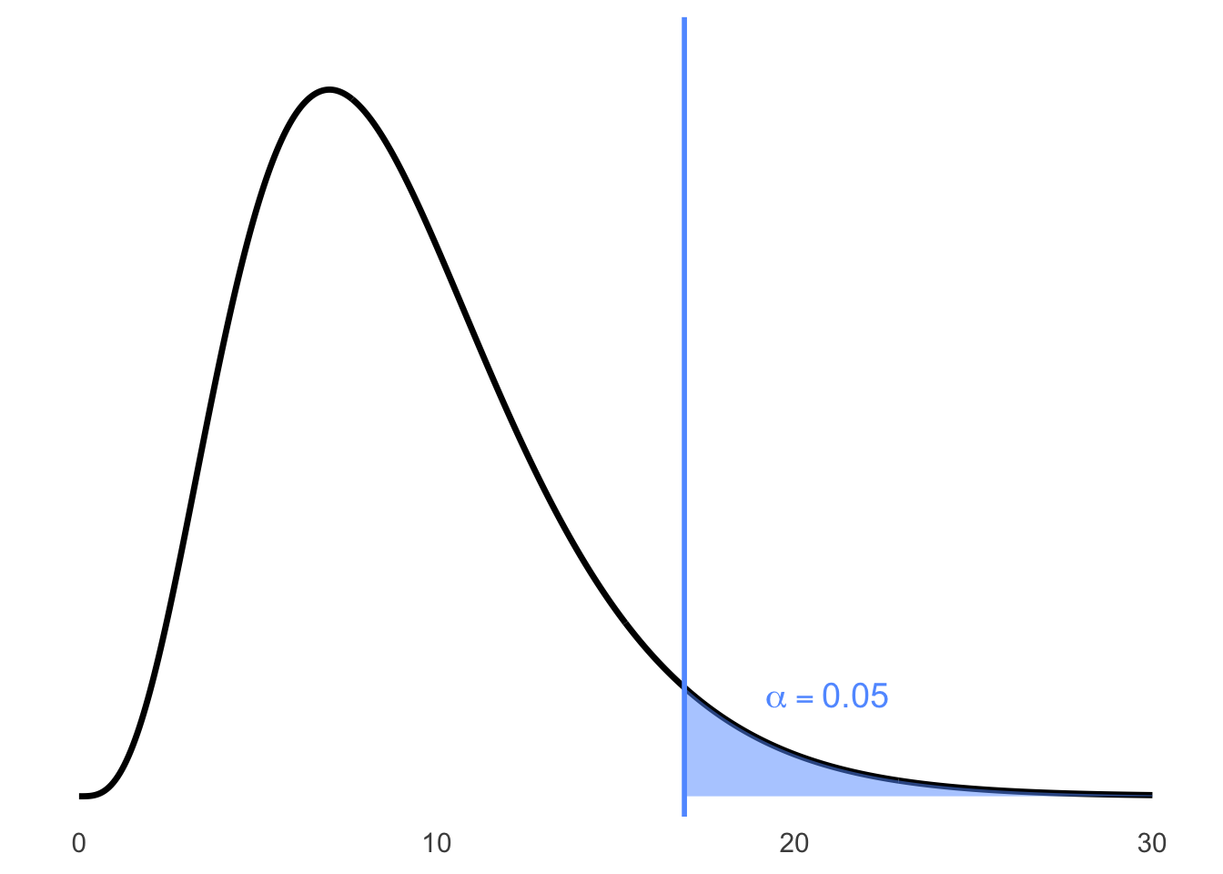
Figure 6.6: Right-tailed chi-squared distribution with critical value at 16.919

Step 4. Conclusion.
The \(\chi^2\) statistic is not significant at the 0.05 level. We conclude that there is insufficient evidence to claim that \(\sigma > 0.9\) year.

6.3 Two Sample Hypothesis Tests

We now move to examining hypothesis tests on 2 independent samples. We will use the notation

\(\Theta_1\) : Parameter of interest from Population 1. \(\Theta_2\) : Parameter of interest from Population 2. \(\Theta_0\) : Numerical value hypothesized under the null hypothesis.

Hypothesis tests of interest on 2 samples are

\(H_0: \Theta_1 - \Theta_2 = \Theta_0\)	vs.	\(H_a: \Theta_1 - \Theta_2 > \Theta_0\)
\(H_0: \Theta_2 - \Theta_2 = \Theta_0\)	vs.	\(H_a: \Theta_1 - \Theta_2 < \Theta_0\)
\(H_0: \Theta_1 - \Theta_2 = \Theta_0\)	vs.	\(H_a: \Theta_1 - \Theta_2 \neq \Theta_0\)

Some other potential hypothesis tests of interest on 2 samples are

\(H_0: \displaystyle\frac{\Theta_1}{\Theta_2} = \Theta_0\)	vs.	\(H_a: \displaystyle\frac{\Theta_1}{\Theta_2} > \Theta_0\)
\(H_0: \displaystyle\frac{\Theta_1}{\Theta_2} = \Theta_0\)	vs.	\(H_a: \displaystyle\frac{\Theta_1}{\Theta_2} < \Theta_0\)
\(H_0: \displaystyle\frac{\Theta_1}{\Theta_2} = \Theta_0\)	vs.	\(H_a: \displaystyle\frac{\Theta_1}{\Theta_2} \neq \Theta_0\)

Remark.

A very common test is to determine whether \(\Theta_1 = \Theta_2\). Therefore, testing

\(H_0: \Theta_1 - \Theta_2 = \Theta_0\)

is equivalent to setting \(\Theta_0 = 0\) and writing the null hypothesis as

\(H_0: \Theta_1 = \Theta_2\)

6.3.1 On a Difference of Means

In this section, our parameter of interest is \(\mu_1 - \mu_2\) where \(\mu_1\) is the mean from one population and \(\mu_2\) is the mean from another population.

6.3.1.1 When \(\sigma_1\) and \(\sigma_2\) are Known

To test \(H_0 : \mu_1 - \mu_2 = \mu_0\), when population variances are unknown and assumed equal, our options for the null and alternative hypotheses are:

• \(H_0: \mu_1 - \mu_2 = \mu_0\) vs. \(H_a: \mu_1 - \mu_2 > \mu_0\)

• \(H_0: \mu_1 - \mu_2 = \mu_0\) vs. \(H_a: \mu_1 - \mu_2 < \mu_0\)

• \(H_0: \mu_1 - \mu_2 = \mu_0\) vs. \(H_a: \mu_1 - \mu_2 \neq \mu_0\)

We calculate the \(z\)-statistic: \[z = \frac{\bar{x}_1 - \bar{x}_2 - \mu_0}{\sqrt{\displaystyle\frac{\sigma_1^2}{n_1} + \frac{\sigma_2^2}{n_2}}}\]

6.3.1.2 When \(\sigma_1\) and \(\sigma_2\) are Not Known

6.3.1.3 When \(\sigma_1 = \sigma_2\)

To test \(H_0 : \mu_1 - \mu_2 = \mu_0\), when population variances are unknown and assumed equal, our options for the null and alternative hypotheses are:

• \(H_0: \mu_1 - \mu_2 = \mu_0\) vs. \(H_a: \mu_1 - \mu_2 > \mu_0\)

• \(H_0: \mu_1 - \mu_2 = \mu_0\) vs. \(H_a: \mu_1 - \mu_2 < \mu_0\)

• \(H_0: \mu_1 - \mu_2 = \mu_0\) vs. \(H_a: \mu_1 - \mu_2 \neq \mu_0\)

We calculate the \(t\)-statistic:

\[z = \frac{\bar{x}_1 - \bar{x}_2 - \mu_0}{\sqrt{\displaystyle\frac{s_1^2}{n_1} + \frac{s_2^2}{n_2}}} \sim t_{\min(n_1 - 1, \, n_2 - 1)}\] where the pooled standard deviation is defined as: \[s_p^2 = \frac{(n_1 - 1)s_1^2 + (n_2 - 1)s_2^2}{n_1 + n_2 - 2}\]

In terms of a variable \(T\) which follows a standard normal distribution, the p-value for a test of \(H_0\) against:

• \(H_a: \mu_1 - \mu_2 > \mu_0\) is \(P(T > z^{*})\)

• \(H_a: \mu_1 - \mu_2 < \mu_0\) is \(P(T < z^{*})\)

• \(H_a: \mu_1 - \mu_2 \neq \mu_0\) is \(2P(T > |z^{*}|)\)

Example 6.16 Comparing Two Population Means Managerial Success Indexes for Two Groups (With Equal Variances Assumed)

Behavioural researchers have developed an index designed to measure managerial success. The index (measured on a 100-point scale) is based on the manager’s length of time in the organization and their level within the term; the higher the index, the more successful the manager. Suppose a researcher wants to compare the average index for the two groups of managers at a large manufacturing plant. Managers in group 1 engage in high volume of interactions with people outside the managers’ work unit (such interaction include phone and face-to-face meetings with customers and suppliers, outside meetings, and public relation work). Managers in group 2 rarely interact with people outside their work unit. Independent random samples of 12 and 15 managers are selected from groups 1 and 2, respectively, and success index of each is recorded.

Response variable: Managerial Success Indexes (quantitative, continuous, 0–100 scale)

Explanatory variable: Type of group (nominal categorical: Group 1 = interaction with outsiders, Group 2 = fewer interactions)

R Code

    # Importing data file into R
    success = read.csv(file = "success.csv", header = TRUE);

    # Getting names of variables
    names(success);

    # Seeing first few observations
    head(success);

    # Attaching data file
    attach(success);

R Code

    ## [1] "Success_Index" "Group"
    ##   Success_Index Group
    ## 1            65     1
    ## 2            66     1
    ## 3            58     1
    ## 4            70     1
    ## 5            78     1
    ## 6            53     1

R code (Descriptive Statistics)

    # loading library mosaic
    library(mosaic)

    favstats(Success_Index ~ Group)

R Code (Descriptive Statistics)

    ## .group min   Q1 median   Q3 max     mean       sd  n
    ##       1  53 62.25  65.50 69.25  78 65.33333 6.610368 12
    ##       2  34 42.50  50.00 54.50  68 49.46667 9.334014 15

R Code (Descriptive Statistics)

    summary(Success_Index[Group == 1]);
    length(Success_Index[Group == 1]);
    sd(Success_Index[Group == 1]);

    summary(Success_Index[Group == 2]);
    length(Success_Index[Group == 2]);
    sd(Success_Index[Group == 2]);

Note: Group 1 = “interaction with outsiders” and Group 2 = “fewer interactions”.

R Output

    ##  Min.  1st Qu.  Median    Mean  3rd Qu.    Max. 
    ##  53.00   62.25   65.50   65.33   69.25   78.00 
    ## [1] 12
    ## [1] 6.610368

    ##  Min.  1st Qu.  Median    Mean  3rd Qu.    Max. 
    ##  34.00   42.50   50.00   49.47   54.50   68.00 
    ## [1] 15
    ## [1] 9.334014

Nearly Normal Condition (Group 1: “interaction with outsiders”):

    stem(Success_Index[Group == 1]);

R Output

    ## 
    ##  The decimal point is 1 digit(s) to the right of the |
    ## 
    ##  5 | 38
    ##  6 | 0335689
    ##  7 | 018

Nearly Normal Condition (Group 2: “fewer interactions”):

    stem(Success_Index[Group == 2]);

R Output

    ## 
    ##  The decimal point is 1 digit(s) to the right of the |
    ## 
    ##  3 | 46
    ##  4 | 22368
    ##  5 | 023367
    ##  6 | 28

Nearly Normal Condition (Group 1: “interaction with outsiders”):

    qqnorm(Success_Index[Group == 1]);
    qqline(Success_Index[Group == 1]);

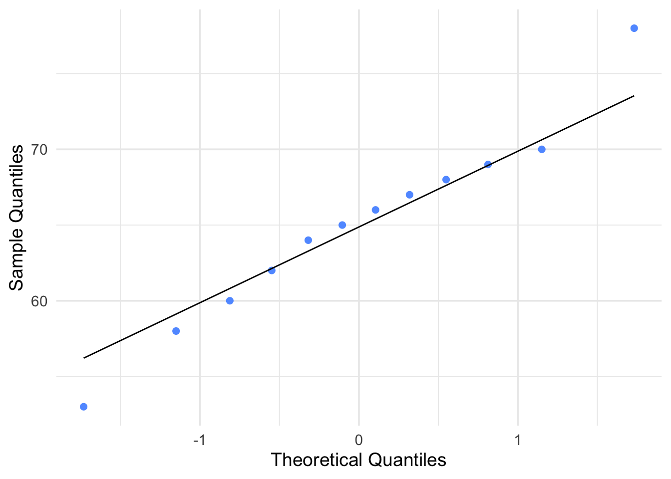
Figure 6.7: Q-Q Plot for Group 1: Interaction with Outsiders

Nearly Normal Condition (Group 2: “fewer interactions”):

    qqnorm(Success_Index[Group == 2]);
    qqline(Success_Index[Group == 2]);

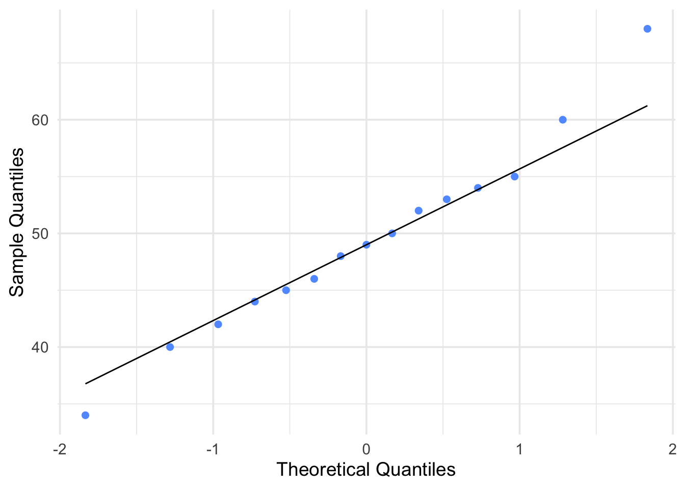
Figure 6.8: Q-Q Plot for Group 2: Fewer Interactions

Nearly Normal Condition:

    boxplot(Success_Index ~ Group, col = c("red", "blue"))

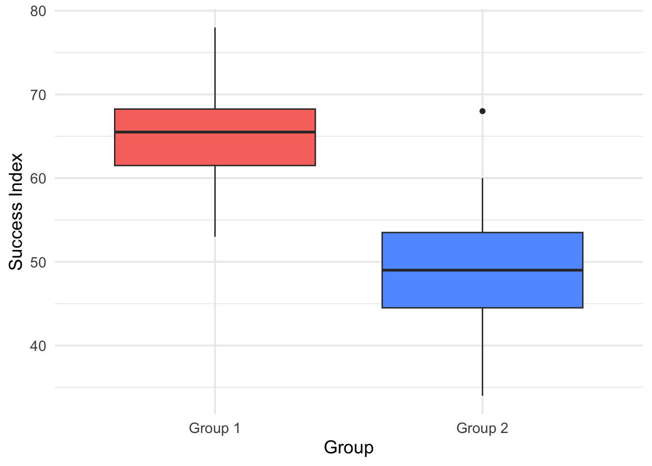
Figure 6.9: Boxplot of Success Index by Group

:::

Boxplot with ggplot2:

    # loading library;
    library(ggplot2);

    # converting a numeric variable into factor (categorical data)
    group <- factor(Group);

    # bp: just a name (not code) to store boxplots;
    bp <- ggplot(success,
                 aes(x = group, y = Success_Index, fill = group));

    our.labs <- c("Interaction with Outsiders", "Fewer Interactions");

    bp +
      geom_boxplot() +
      scale_x_discrete(labels = our.labs);

Checking the Assumptions and Conditions

Independent Group Assumption: The success index in group 1 is unrelated to the success index in group 2.

Randomization Condition: The 27 managers were randomly and independently selected (12 for group 1, and 15 for group 2).

Nearly Normal Condition: The two boxplots of success indexes do not show skewness; the two stemplots/histograms of success indexes are unimodal, fairly symmetric and approximately bell-shaped. Q–Q plots also suggest the normality assumption is reasonable.

Equal Variances Assumption: The two boxplots of success indexes appear to have the same spread; thus, the samples appear to have come from populations with approximately the same variance.

Since the conditions are satisfied, it is appropriate to construct a \(t\) confidence interval with
\(df = 12 + 15 - 2 = 25\).
From the data, the following statistics were calculated:

\[\begin{aligned} n_1 &= 12 &\quad n_2 &= 15 \\ \bar{x}_1 &= 65.33 &\quad \bar{x}_2 &= 49.47 \\ s_1^2 &= 6.61^2 &\quad s_2^2 &= 9.33^2 \end{aligned}\]

The pooled variance estimator is:

\[s_p^2 = \frac{(n_1 - 1)s_1^2 + (n_2 - 1)s_2^2}{n_1 + n_2 - 2} = \frac{(12 - 1)(6.61^2) + (15 - 1)(9.33^2)}{12 + 15 - 2} = 67.97\]

The number of degrees of freedom is: \[\nu = n_1 + n_2 - 2 = 12 + 15 - 2 = 25\]

6.3.1.4 When \(\sigma_1 \neq \sigma_2\)

To test \(H_0 : \mu_1 - \mu_2 = \mu_0\), when population variances are unknown and assumed different, our options for the null and alternative hypotheses are:

• \(H_0: \mu_1 - \mu_2 = \mu_0\) vs. \(H_a: \mu_1 - \mu_2 > \mu_0\)

• \(H_0: \mu_1 - \mu_2 = \mu_0\) vs. \(H_a: \mu_1 - \mu_2 < \mu_0\)

• \(H_0: \mu_1 - \mu_2 = \mu_0\) vs. \(H_a: \mu_1 - \mu_2 \neq \mu_0\)

We calculate the \(t\)-statistic:

\[t^* = \frac{\bar{x}_1 - \bar{x}_2 - \mu_0}{\sqrt{\frac{s_1^2}{n_1} + \frac{s_2^2}{n_2}}} \sim t_{\min(n_1 -1, n_2 -1)}\]

In terms of a variable \(T\) which follows a standard normal distribution, the p-value for a test of \(H_0\) against:

• \(H_a: \mu_1 - \mu_2 > \mu_0\) is \(P(T > z^{*})\)

• \(H_a: \mu_1 - \mu_2 < \mu_0\) is \(P(T < z^{*})\)

• \(H_a: \mu_1 - \mu_2 \neq \mu_0\) is \(2P(T > |z^{*}|)\)

Remark. Note a more accurate approximation of the degrees of freedom is given by \[df = \frac{\left( \frac{s_1^2}{n_1} + \frac{s_2^2}{n_2} \right)^2} { \left( \frac{1}{n_1 - 1} \left( \frac{s_1^2}{n_1} \right)^2 \right) + \left( \frac{1}{n_2 - 1} \left( \frac{s_2^2}{n_2} \right)^2 \right) }\]

This approximation is accurate when both sample sizes \(n_1\) and \(n_2\) are 5 or larger.

Example 6.17 “Conservationists have despaired over destruction of tropical rain forest by logging, clearing, and burning”. These words begin a report on a statistical study of the effects of logging in Borneo. Here are data on the number of tree species in 12 unlogged forest plots and 9 similar plots logged 8 years earlier:

Unlogged: 22 18 22 20 15 21 13 13 19 13 19 15
Logged : 17 4 18 14 18 15 15 10 12

Does logging significantly reduce the mean number of species in a plot after 8 years? State the hypotheses and do a t test. Is the result significant at the 5% level?
Solution:
1. State hypotheses. \(H_0: \mu_1 = \mu_2\) vs. \(H_a: \mu_1 > \mu_2\), where \(\mu_1\) is the mean number of species in unlogged plots and \(\mu_2\) is the mean number of species in plots logged 8 years earlier.

2. Test statistic. \[t^* \;=\;\frac{\bar x_1 - \bar x_2}{\sqrt{s_1^2/n_1 + s_2^2/n_2}} \;=\;2.1140\] \[(\bar x_1 = 17.5,\;\bar x_2 = 13.6666,\;s_1 = 3.5290,\;s_2 = 4.5,\;n_1 = 12,\;n_2 = 9)\]

3. P-value. Using Table, we have \(df = 8\), and \(0.025 < \text{P-value} < 0.05\).

4. Conclusion. Since P-value \(< 0.05\), we reject \(H_0\). There is strong evidence that the mean number of species in unlogged plots is greater than that for logged plots 8 years after logging.

Example 6.18 A company that sells educational materials reports statistical studies to convince customers that its materials improve learning. One new product supplies “directed reading activities” for classroom use. These activities should improve the reading ability of elementary school pupils.

A consultant arranges for a third-grade class of 21 students to take part in these activities for an eight-week period. A control classroom of 23 third-graders follows the same curriculum without the activities. At the end of the eight weeks, all students are given a Degree of Reading Power (DRP) test, which measures the aspects of reading ability that the treatment is designed to improve. The data appear in the following table.

Treatment				Control
24	61	59	46	42	33	46	37
43	44	52	43	43	41	10	42
58	67	62	57	55	19	17	55
71	49	54		26	54	60	28
43	53	57		62	20	53	48
49	56	33		37	85	42

Because we hope to show that the treatment (Group 1) is better than the control (Group 2), the hypotheses are:

\[H_0 : \mu_1 = \mu_2\] \[H_a : \mu_1 > \mu_2\]

    # Step 1. Entering data
    treatment = c(24, 61, 59, 46, 43, 44, 52, 43, 58, 67, 62, 57, 
                  71, 49, 54, 43, 53, 57, 49, 56, 33);
    control = c(42, 33, 46, 37, 43, 41, 10, 42, 55, 19, 17, 55, 
                26, 54, 60, 28, 62, 20, 53, 48, 37, 85, 42);

Nearly Normal Condition (treatment):

    # Making stemplot;

    stem(treatment);

    ##
    ## The decimal point is 1 digit(s) to the right of the |
    ##
    ## 2 | 4
    ## 3 | 3
    ## 4 | 3334699
    ## 5 | 23467789
    ## 6 | 127
    ## 7 | 1

Nearly Normal Condition (control):

    # Making stemplot;

    stem(control);

    ##
    ## The decimal point is 1 digit(s) to the right of the |
    ##
    ## 0 | 079
    ## 2 | 068377
    ## 4 | 12223683455
    ## 6 | 02
    ## 8 | 5

Nearly Normal Condition (treatment):

    # Making Q-Q plot;
    qqnorm(treatment, pch=19, col="red", main="Treatment");
    qqline(treatment, lty=2);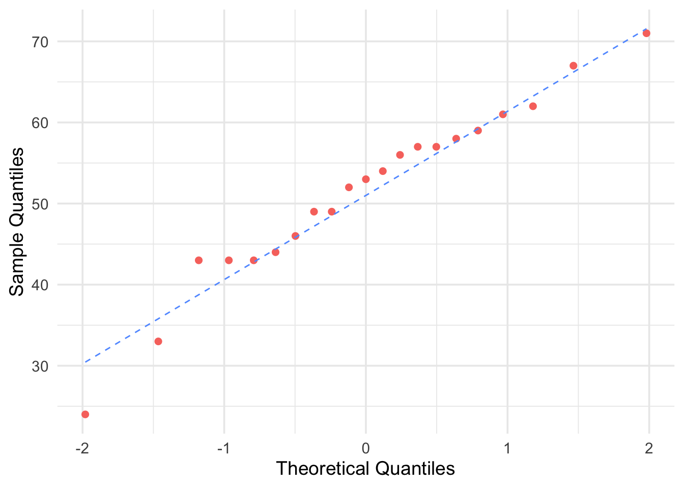

Figure 6.10: Q-Q Plot for Treatment Group

Nearly Normal Condition (control):

    # Making Q-Q plot;
    qqnorm(treatment, pch=19, col="red", main="Control");
    qqline(control, lty=2);

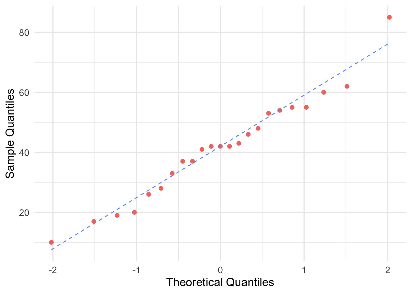
Figure 6.11: Q-Q Plot for Control Group

Stemplots suggest that there is a mild outlier in the control group but no deviation from Normality serious enough to prevent us from using t procedures. Normal Q-Q plots for both groups confirm that both are roughly Normal. The summary statistics are:

    summary(treatment);

    ## Min. 1st Qu.  Median    Mean 3rd Qu.    Max. 
    ## 24.00   44.00   53.00   51.48   58.00   71.00

    summary(control);

    ## Min. 1st Qu.  Median    Mean 3rd Qu.    Max. 
    ## 10.00   30.50   42.00   41.52   53.50   85.00

    # Step 1. Entering data;

    treatment = c(24, 61, 59, 46, 43, 44, 52, 43, 58, 67, 62, 57, 
                  71, 49, 54, 43, 53, 57, 49, 56, 33);
                  
    control = c(42, 33, 46, 37, 43, 41, 10, 42, 55, 19, 17, 55, 
                26, 54, 60, 28, 62, 20, 53, 48, 37, 85, 42);

    # Step 2. Hypothesis Test

    t.test(treatment, control, alternative="greater")

Hypothesis Test (using R)

    ##
    ##  Welch Two Sample t-test
    ## 
    ## data:  treatment and control
    ## t = 2.3106, df = 37.855, p-value = 0.01305
    ## alternative hypothesis: true difference in means is greater than 0
    ## 95 percent confidence interval:
    ##  2.333784      Inf
    ## sample estimates:
    ## mean of x mean of y 
    ##    51.47619 41.52174 

Hypothesis Test (using table)

    round (mean(treatment) ,2);

    ##[1] 51.48

    round (sd(treatment) ,2);

    ##[1] 11.01

    round (mean(control) ,2);

    ##[1] 41.52

    round (sd(control) ,2);

    ##[1] 17.15

Test statistic.
\[t^* = \frac{\bar{x}_1 - \bar{x}_2}{\sqrt{\frac{s_1^2}{n_1} + \frac{s_2^2}{n_2}}} = 2.31\] \[\quad (\bar{x}_1 = 51.48, \, \bar{x}_2 = 41.52, \, s_1 = 11.01, \, s_2 = 17.15, \quad n_1 = 21 \text{ and } n_2 = 23)\]

The conservative approach uses the t(20) distribution. The P-value for the one-sided test is \[\text{P-value} = P\bigl(T \geq 2.31 \bigr)\] Comparing \(t = 2.31\) with the entries in Table 5 for 20 degrees of freedom, we see that \[0.01 < \text{P-value} < 0.025.\]

Since our P-value is “small”, we reject the null hypothesis (Note that we would reject \(H_0\) at the 2.5% significance level). The data strongly suggest that directed reading activity improves the DRP score.

The design of the DRP study is not ideal. Random assignment of students was not possible in a school environment, so existing third-grade classes were used. The effect of the reading programs is therefore confounded with any other differences between the two classes. The classes were chosen to be as similar as possible in variables such as the social and economic status of the students. Pretesting showed that the two classes were on the average quite similar in reading ability at the beginning of the experiment. To avoid the effect of two different teachers, the same teacher taught reading in both classes during the eight-week period of the experiment. We can therefore be somewhat confident that our two-sample procedure is detecting the effect of the treatment and not some other difference between the classes.

Remark. The Fold Rule

A rule which can be used to quickly determine whether population variances are equal or unequal using sample variances.

If \[\frac{\max(s_1, s_2)}{\min(s_1, s_2)} < \sqrt{2} \quad \text{then we can consider } \sigma_1^2 = \sigma_2^2\]

and

\[\frac{\max(s_1^2, s_2^2)}{\min(s_1^2, s_2^2)} < 2 \quad \text{then we can consider } \sigma_1^2 = \sigma_2^2\]

This is quick and simple technique. It is only a rule and not as strong as conducting the hypothesis tests for equality of varianges

\[H_0: \sigma_1^2 = \sigma_2^2 \quad \text{vs} \quad H_a: \sigma_1^2 \neq \sigma_2^2\] which was covered in Section 6.3.3

6.3.1.5 Assumptions

6.3.2 On a Difference of Proportions

We can use hypothesis test to compare proportions from two independent groups as well.

To test \(H_0 : p_1 - p_2 = p_0\), our options for the null and alternative hypotheses are:

• \(H_0: p_1 - p_2 = p_0\) vs. \(H_a: p_1 - p_2 > p_0\)

• \(H_0: p_1 - p_2 = p_0\) vs. \(H_a: p_1 - p_2 < p_0\)

• \(H_0: p_1 - p_2 = p_0\) vs. \(H_a: p_1 - p_2 \neq p_0\)

We calculate the \(z\)-statistic:

\[z_* = \frac{\hat{p_1} - \hat{p_2} - p_0}{\sqrt{\hat{p}(1-\hat{p})\left(\displaystyle\frac{1}{n_1}+ \frac{1}{n_2}\right)}} \sim N(0,1).\]

where

\[\hat{p} = \frac{x_1 + x_2}{n_1+n_2}\]

and \(n_1\) and \(n_2\) represent sample sizes of each group.

In terms of a variable \(Z\) which follows a standard normal distribution, the p-value for a test of \(H_0\) against:

• \(H_a: p_1 - p_2 > p_0\) is \(P(Z > z^{*})\)

• \(H_a: p_1 - p_2 < p_0\) is \(P(Z < z^{*})\)

• \(H_a: p_1 - p_2 \neq p_0\) is \(2P(Z > |z^{*}|)\)

Example 6.19 Nicotine patches are often used to help smokers quit. Does giving medicine to fight depression help? A randomized double-blind experiment assigned 244 smokers who wanted to stop to receive nicotine patches and another 245 to receive both a patch and the anti-depression drug bupropion. Results: After a y ear, 40 subjects in the nicotine patch group had abstained from smoking, as had 87 in the patch-plus-drug group. How significant is the evidence that the medicine increases the success rate? State hypotheses, calculate a test statistic, use Table 6 to give its P-value, and state y our conclusion. (Use \(\alpha = 0.01\))
Solution:

Step 1: State Hypothesis

\(H_0: p_1 = p_2\) and \(H_a: p_1 < p_2\)

Step 2: Find test statistics

\(\hat{p_1} = \frac{40}{244} = 0.1639\) and \(\hat{p_2} = \frac{87}{245} = 0.3551\). Then \(\hat{p} = \frac{40+87}{244+245} = 0.2597\).

Now, \(z_* = \frac{\hat{p_1} - \hat{p_2}}{\sqrt{\hat{p}(1-\hat{p})(\frac{1}{n_1} + \frac{1}{n_2})}} = -4.82\)

Step 3: Compute p-value

P-value \(= P(Z < z_*) = P(Z < -4.82) < 0.0003\)

Step 4: Conclusion

Since p-value \(< 0.0003 < \alpha = 0.01\), we reject the null hypothesis that \(p_1 = p_2\). The data provide very strong evidence that bupropion increases success rate.

R-code:

Input

successes=c(87, 40);

totals=c(245, 244);

prop.test(successes, totals, alternative="greater",correct=FALSE);

Output

## 
## 2-sample test for equality of proportions without 
## continuity correction 
## 
## data: x and n
## X-squared = 23.237, df = 1, p-value = 7.161e-07
## alternative hypothesis: greater 
## 95 percent confidence interval: 
## 0.1275385 1.0000000 
## sample estimates:
##    prop 1    prop 2 
## 0.3551020 0.1639344

6.3.2.1 Assumptions

• Independent Response Assumption: Within each group , we need independent responses from the cases. We cannot check that for certain, but randomization provides evidence of independence. So, we need to check the following:

  • Randomization Condition: The data in each group should be drawn independently and at random from a population or generated by a completely randomized designed experiment.

  • The 10 % Condition: If the data are sampled without replacement, the sample should not exceed 10 % of the population. If samples are bigger than 10 % of the target population, random draws are no longer approximately independent.

  • Independent Groups Assumption: The two groups we are comparing must be independent from each other.

• Sample Size Condition Each of the groups must be big enough. As with individual proportions, we need larger group s to estimate proportions that are near 0% and 100%. We check the success / failure condition for each group.

  • Success / Failure Condition: Both groups are big enough that at least 10 successes and at least 10 failures have been observed in each group or will be expected in each (when testing hypothesis).

6.3.3 On a Ratio of Variances

Let’s begin this type of hypothesis test with a case. The question is: how do you know whether the homogeneity of variance assumption is satisfied? One simple method involves just looking at two sample variances. Logically, if two population variances are equal, then the two sample variances should be very similar. When the two sample variances are reasonably close, you can be reasonably confident that the homogeneity assumption is satisfied and proceed with, for example, Student t-interval. However, when one sample variance is three or four times larger than the other, then there is reason for a concern. The common statistical procedure for comparing population variances \(\sigma_1^2\) and \(\sigma_2^2\) makes an inference about the ratio of \(\sigma_1^2\)/\(\sigma_2^2\).

To test \(H_0 : \mu_d = \mu_0\), our options for the null and alternative hypotheses are:

• \(H_0: \sigma_1^2 = \sigma_2^2\) vs. \(H_a: \sigma_1^2 > \sigma_2^2\)

• \(H_0: \sigma_1^2 = \sigma_2^2\) vs. \(H_a: \sigma_1^2 < \sigma_2^2\)

• \(H_0: \sigma_1^2 = \sigma_2^2\) vs. \(H_a: \sigma_1^2 \neq \sigma_2^2\)

We calculate the \(F\)-statistic:

\[F^{*} = \frac{s_1^2}{s_2^2} \sim F_{n_1-1,n_2-1}.\]

In terms of a variable \(F\) which follows an \(F\)-distribution with \(n_1-1\) and \(n_2-1\) degrees of freedom, the p-value for a test of \(H_0\) against:

• \(H_a: \sigma_1^2 > \sigma_2^2\) is \(P(F > F^{*})\)

• \(H_a: \sigma_1^2 < \sigma_2^2\) is \(P(F < F^{*})\)

• \(H_a: \sigma_1^2 \neq \sigma_2^2\) is \(2P(F > |F^{*}|)\)

6.3.3.1 Assumptions

• The two samples are independent.
• The populations from which the samples are drawn are normally distributed.
• The data are measured on a continuous scale.

6.4 Hypothesis Tests on Paired Data

When observations in sample 1 matches with an observation in sample 2. Observations in sample 1 are, usually, highly, correlated with observations in sample 2, these data are often called matched pairs. For each pair (the same cases), we form: Difference = observation in sample 2 - observation in sample 1. Thus, we have one single sample of differences scores. For example, in longitudinal studies: Pre- and post-survey of attitudes towards statistics (Same student is measured twice: Time 1 (pre) and Time 2 (post). We measure change in the attitudes: Post - Pre (for each student). Often these types of studies are called, repeated measures.
Paired Data Condition: the data must be quantitative and paired.
Independence Assumption:

• If the data are paired, recall the measurements are not independent since 2 measurements are taken on each unit. However, since each unit is sampled independently, the differences must be independent of each other.

• The pairs should be a random sample.

• In experimental design, the order of the two treatments may be randomly assigned, or the treatments ma y be randomly assigned to one member of each pair.

• In a before-and-after study, we may believe that the observed differences are representative sample of a population of interest. If there is any doubt, we need to include a control group to be able to draw conclusions.

• If samples are bigger than 10 % of the target population, we need to acknowledge this and note in our report. When we sample from a finite population, we should be careful not to sample more than 10 % of that population. Sampling too large a fraction of the population calls the independence assumption into question.

Recall Section 5.5 where we covered confidence intervals on paired data, we introduced the table below:

Sample Units	Measurement 1 (\(M_{1}\))	Measurement 2 (\(M_{2}\))	Difference (\(M_{2}-M_{1}\))
1	\(x_{11}\)	\(x_{12}\)	\(x_{d1} = x_{12} - x_{11}\)
2	\(x_{21}\)	\(x_{22}\)	\(x_{d2} = x_{22} - x_{21}\)
3	\(x_{31}\)	\(x_{32}\)	\(x_{d3} = x_{32} - x_{31}\)
\(\vdots\)	\(\vdots\)	\(\vdots\)	\(\vdots\)
n	\(x_{n1}\)	\(x_{n2}\)	\(x_{dn} = x_{n2} - x_{n1}\)

From that table, we can get \(\bar{x}_{d}\), which is the mean, variance and standard deviation of the difference. We need these values to continue our analysis.

To test \(H_0 : \mu_d = \mu_0\), our options for the null and alternative hypotheses are:

• \(H_0: \mu_d = \mu_0\) vs. \(H_a: \mu_d > \mu_0\)

• \(H_0: \mu_d = \mu_0\) vs. \(H_a: \mu_d < \mu_0\)

• \(H_0: \mu_d = \mu_0\) vs. \(H_a: \mu_d \neq \mu_0\)

We calculate the \(t\)-statistic:

\[t^* = \dfrac{\bar{x}_{d} - \mu_0}{s_{d} / \sqrt{n}} \sim t_{n-1}\] In terms of a variable \(T\) which follows a \(t\)-distribution at \(n-1\) degrees of freedom, the p-value for a test of \(H_0\) against:

• \(H_a: \mu > \mu_0\) is \(P(T > t^{*})\)

• \(H_a: \mu < \mu_0\) is \(P(T < t^{*})\)

• \(H_a: \mu \ne \mu_0\) is \(2P(T > |t^{*}|)\)

Example 6.20 In an effort to determine whether a new type of fertilizer is more effective than the type currently in use, researchers took 12 two-acre plots of land scattered throughout the county. Each plot was divided into two equal-size sub plots, one of which was treated with the new fertilizer. Wheat was planted, and the crop yields were measured.

Plot	1	2	3	4	5	6	7	8	9	10	11	12
Current	56	45	68	72	61	69	57	55	60	72	75	66
New	60	49	66	73	59	67	61	60	58	75	72	68

Can we conclude at the 5% significance level that the new fertilizer is more effective than the current one?

Solution:

You can verify that the mean and standard deviation of the twelve difference measurements are \(\bar{x}_{d} = new - current = 1\) and \(s_d = 3.0151\).

Step 1: State Hypothesis

\(H_0: \mu_d = 0\) and \(H_a: \mu_d>0\)

Step 2: Find test statistics

\(t^{*} = \displaystyle\frac{\bar{x}_{d} - 0}{s_d/\sqrt{n}} = \frac{1}{3.0151/\sqrt{12}} = 1.1489\)

Step 3: Compute p-value

Using t-distribution table with df \(=11\), then \(0.10 < p-value < 0.15\).

Step 4: Conclusion

Since p-value \(> \alpha = 0.05\), we can’t reject \(H_0\). There is not enough evidence to infer that the new fertilizer is better.

6.4.0.1 Assumptions

• The differences between paired observations are approximately normally distributed.
• The samples are randomly and independently drawn from the population.