Chapter 4 Foundations of Inference
The aim of statistical inference is to produce estimators of the population parameters based on a smaller sample and to quantify the accuracy of these estimators in terms of a probability statement. In other words we are interested in the values of unknown parameters for a population thus we collect data from a sample and calculate statistics to estimate the parameters of interest. We then quantify our confidence that the statistic is representative of the parameter.
Statistical inference is concerned primarily with understanding the quality of parameter estimates. For example, a classic inferential question is, “How sure are we that the estimated mean, \(\bar{x}\), is near the true population mean, \(\mu\)?” While the equations and details change depending on the setting, the foundations for inference are the same throughout all of statistics.
4.1 Some Important Statistical Distributions
4.1.1 Introduction to the Normal Distribution
In probability theory and statistics, the normal distribution is one of the most important distribution used to model many populations and processes which occur in reality.
Definition 4.1 (Normal distribution) Let \(X\) be a random variable with mean \(-\infty < \mu < +\infty\) and variance \(\sigma^2 > 0\). We say that \(X\) folowes a normal distribution if the probability density function of \(X\) is: \[f(x) = \frac{1}{\sqrt{2 \pi \sigma^2}} \cdot e^{-\displaystyle\frac{(x - \mu)^2}{2\sigma^2}}, \text{ for $-\infty < x < \infty$.}\]
Remark. The normal distribution is also called Gaussian distribution since it was discovered Johann Carl Friedrich Gauss in 1809. Gauss is one of the most influential and important mathematicians in history.
The normal distribution is symmetric about its mean \(\mu\) and has a bell-shaped curve. It is completely characterized by two parameters which are the the mean \(\mu\) and the standard deviation \(\sigma\). Some examples are shown in Figure 4.1.
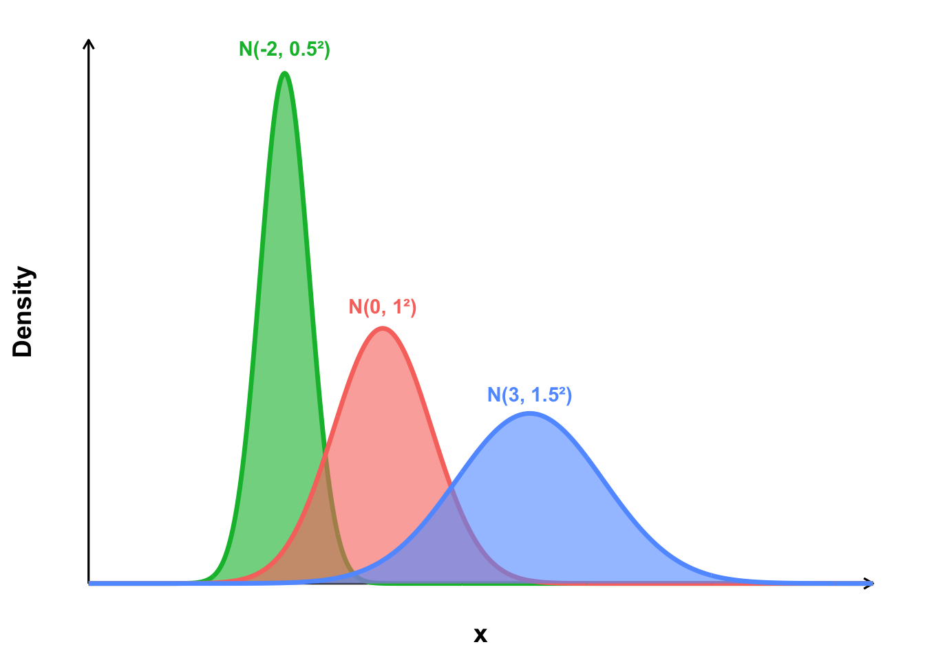
Figure 4.1: Some examples of normal distrubution curves with different means and variances
A special case of normal distribution is standard normal distribution which is explained in Definition 4.2.
Definition 4.2 (Standard normal distribution) Let \(Z \sim N( \mu = 0, \sigma^2 = 1)\), then \(Z\) has probability density function as: \[f(y) = \frac{1}{\sqrt{2\pi}} \cdot e^{-\displaystyle\frac{z^2}{2}}.\] which is called the standard normal distribution.
Remark. Standard normal random variables are often denoted by \(Z\).
A useful property of the normal distribution is that it is symmetric about its mean \(\mu\).
Remark. The Empirical Rule informs us that for any symmetric (bell-shaped) curve, let \(\mu\) be its mean and \(\sigma\) be its standard deviation, the following probability set function is true:
\(1.\) \(P(\mu - \sigma < X < \mu + \sigma) = 68.27\%;\)
\(2.\) \(P(\mu - 2\sigma < X < \mu + 2\sigma) = 95.45\%;\)
\(3.\) \(P(\mu - 3\sigma < X < \mu + 3\sigma) = 99.73\%.\)
The interactive application below illustrates the empirical rule.
Remark. A consequence of the Empirical Rule from 4.1.1 is that for a sample drawn from a population that is approximately normal, we can roughly estimate the standard deviation using the crude approximate :
\[\hat{\sigma} \approx \frac{\text{Sample Range}}{4}.\]
4.1.2 Introduction to the Chi-Square distribution
Before we introduce the chi-Square square distribution, we recall the gamma distribution.
Definition 4.3 (Gamma distribution) A random variable \(X\) is said to follow a Gamma distribution with shape parameter \(\alpha > 0\) and scale parameter \(\beta > 0\) (denoted \(X \sim \mathrm{Gamma}(\alpha,\beta)\)) if its probability density function is \[ f_{X}(x; \alpha, \beta) \;=\; \begin{cases} \dfrac{1}{\Gamma(\alpha)\,\beta^{\alpha}}\,x^{\alpha - 1}\,e^{-x/\beta}, & x > 0, \\[1em] 0, & \text{otherwise}, \end{cases} \] where \(\Gamma(\alpha) = \displaystyle\int_{0}^{\infty} t^{\alpha - 1} e^{-t}\,dt\) is the Gamma function.
The Chi-square random variable follows a Chi-square distribution with \(k\) degrees of freedom if it is defined as the sum of the squares of \(k\) independent standard normal random variables.
Definition 4.4 (Chi-square random variable) A chi-square random variable with \(k\) degrees of freedom is defined as the sum of the squares of \(k\) independent standard normal random variables. Formally, if \[ Z_{1}, Z_{2}, \dots, Z_{k} \;\overset{\mathrm{iid}}{\sim}\; N(0,1), \] then \[ X \;=\;\sum_{i=1}^{k} Z_{i}^{2} \] follows a chi-square distribution with \(k\) degrees of freedom, denoted \(X \sim \chi^{2}_{k}\) and has the probability density function \[ f_{X}(x; k) \;=\; \begin{cases} \dfrac{1}{2^{\,k/2}\,\Gamma\!\bigl(\tfrac{k}{2}\bigr)}\,x^{\,\tfrac{k}{2}-1}\,e^{-x/2}, & x > 0, \\[1em] 0, & \text{otherwise}. \end{cases} \] Where \(\Gamma(\cdot)\) is the Gamma function in Definition 4.3.
The definition of a chi-square random variable can be proven using moment generating functions.
Remark. The Chi-square distribution is also a special case of the gamma distribution, however we will not be covering the gamma distribution in this course.
The shape of the chi-square distribution is determined by its degrees of freedom. Some examples of chi-square distributions are shown in Figure 4.2.
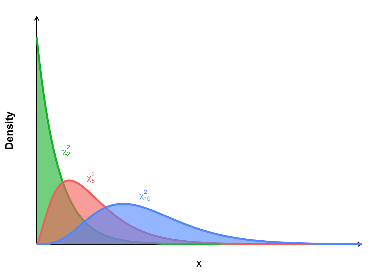
Figure 4.2: Some examples of chi-square distrubution curves with different degrees of freedom
4.1.3 Introduction to the t-Distribution
Definition 4.5 (Student’s (t) Distribution) A Student’s \(t\) random variable with \(\nu\) degrees of freedom is defined as the ratio of a standard normal variate and the square root of a scaled chi-square variate. Formally, if \[ Z \;\overset{\mathrm{iid}}{\sim}\; N(0,1) \quad\text{and}\quad U \;\overset{\mathrm{iid}}{\sim}\; \chi^{2}_{\nu} \] are independent, then \[ T \;=\;\frac{Z}{\sqrt{\,U / \nu\,}} \] follows a Student’s \(t\) distribution with \(\nu\) degrees of freedom, denoted \[ T \sim t_{\nu}, \] and has the probability density function \[ f_{T}(t; \nu) \;=\; \frac{\Gamma\!\bigl(\tfrac{\nu+1}{2}\bigr)}{\sqrt{\pi\,\nu}\,\Gamma\!\bigl(\tfrac{\nu}{2}\bigr)} \Bigl(1 + \tfrac{t^{2}}{\nu}\Bigr)^{-\tfrac{\nu+1}{2}}, \quad -\infty < t < \infty. \] Here \(\Gamma(\cdot)\) is the Gamma function as in Definition 4.3.
The t-distribution resembles the normal distribution but with heavier tails.
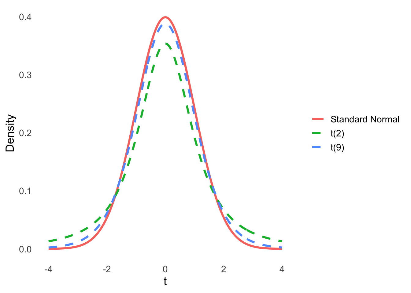
Figure 4.3: Comparison of the standard normal distribution and t-distributions with 2 and 9 degrees of freedom
4.1.4 Introduction to the F-Distribution
Definition 4.6 (Beta function) The Beta function, also called the Euler integral of the first kind, is defined for complex numbers \(\;z_{1}, z_{2}\) with \(\Re(z_{1}), \Re(z_{2})>0\) by the integral \[ B(z_{1}, z_{2}) = \int_{0}^{1} t^{\,z_{1}-1}\,(1 - t)^{\,z_{2}-1}\,\mathrm{d}t. \]
Definition 4.7 (F random variable) An \(F\) random variable with \(\nu_{1}\) and \(\nu_{2}\) degrees of freedom is defined as the ratio of two independent chi-square variates, each divided by its degrees of freedom. Formally, if
\[
U \;\overset{\mathrm{iid}}{\sim}\;\chi^{2}_{\nu_{1}}
\quad\text{and}\quad
V \;\overset{\mathrm{iid}}{\sim}\;\chi^{2}_{\nu_{2}}
\]
are independent, then
\[
F \;=\;\frac{\,U / \nu_{1}\,}{\,V / \nu_{2}\,}
\]
follows an \(F\) distribution with \(\nu_{1}\) and \(\nu_{2}\) degrees of freedom, denoted
\[
F \sim F_{\nu_{1},\nu_{2}},
\]
and has probability density function
\[
f_{F}(x; \nu_{1}, \nu_{2})
=
\begin{cases}
\displaystyle
\frac{\bigl(\tfrac{\nu_{1}}{\nu_{2}}\bigr)^{\!\nu_{1}/2}
\,x^{\,\tfrac{\nu_{1}}{2}-1}}
{B\!\bigl(\tfrac{\nu_{1}}{2},\,\tfrac{\nu_{2}}{2}\bigr)}
\,
\Bigl(1 + \tfrac{\nu_{1}}{\nu_{2}}\,x\Bigr)^{-\tfrac{\nu_{1}+\nu_{2}}{2}},
& x > 0 \\[1em]
0,
& \text{otherwise}.
\end{cases}
\]
where \(B(\cdot,\cdot)\) is the Beta function (see Definition 4.6).
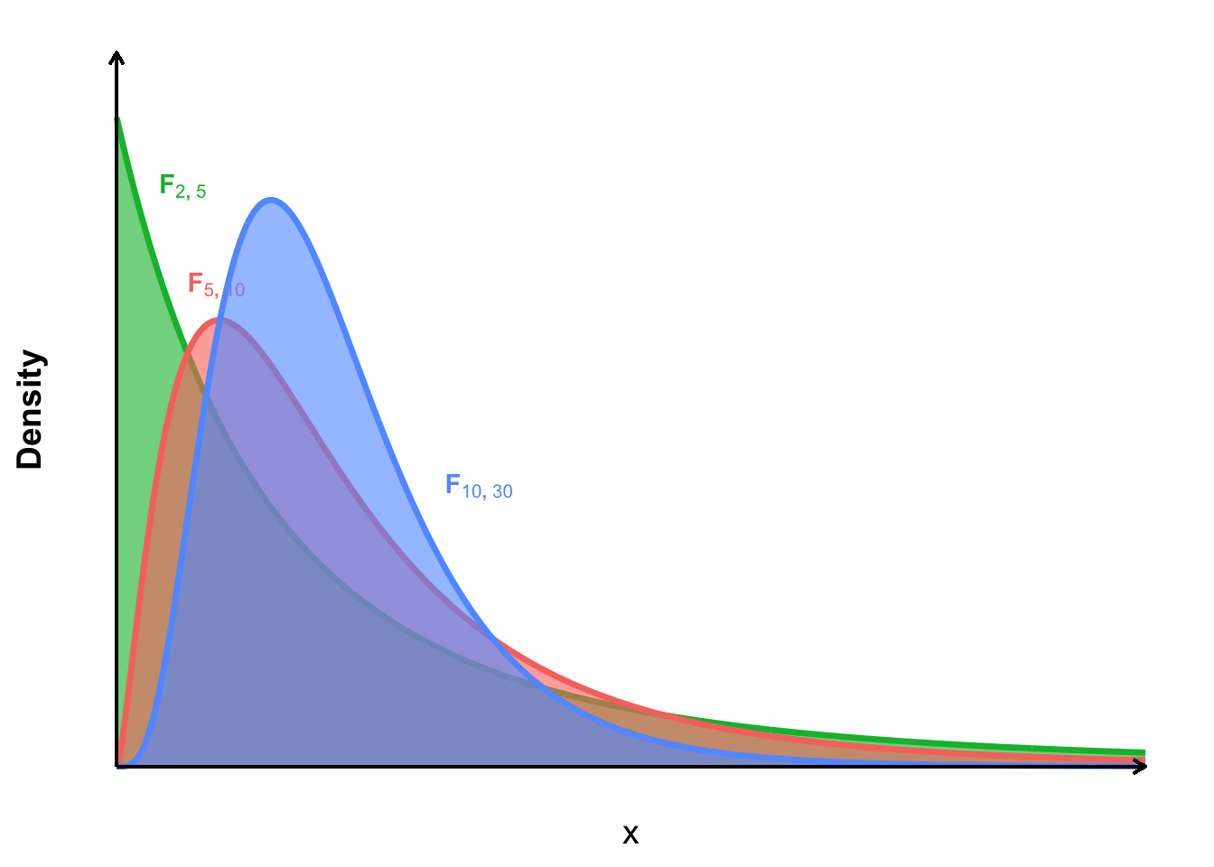
Figure 4.4: The F-Distribution at different degrees of freedom.
4.2 Sampling Distributions
Although this may be a new concept, a statistic can follow a distribution. The distribution of a statistic is called its sampling distribution.
Definition 4.8 (Sampling distribution) The sampling distribution of a statistic is the probability distribution of that statistic computed from all possible random samples of a given size drawn from the same population.
In other words, Definition 4.8 in informing us that if we repeatedly draw samples of size \(n\) and compute the statistic (e.g. the sample mean \(\bar X\)), then the values of \(\bar X\) across those samples form a distribution, which is its sampling distribution. The sampling distribution is important because it allows us to understand the variability of a statistic from sample to sample, and it forms the basis for inferential statistics, such as confidence intervals and hypothesis tests.
4.3 The Central Limit Theorem
The central limit theorem (CLT) explains why the distribution of a properly standardized sample mean becomes approximately normal as the sample size grows—even when the underlying population is not normal.
Suppose \(X_1,X_2,\dots,X_n\) are independent and identically distributed (i.i.d.) with finite mean \(\mu\) and variance \(\sigma^{2}\). Define the sample mean \(\bar X_n = \tfrac{1}{n}\sum_{i=1}^{n} X_i\). The Centrel Limit Theorem tells us that the random fluctuation of \(\bar X_n\) around the population mean \(\mu\) (after appropriate scaling) behaves more and more like a standard normal variable as \(n\) increases.
Theorem 4.1 (Central Limit Theorem) Let \(X_{1},X_{2},\dots,X_{n}\) be i.i.d. random variables with
\(E[X_i]=\mu\) and \(\operatorname{Var}(X_i)=\sigma^{2}<\infty\).
Then, as \(n\to\infty\),
\[ \frac{\sqrt{n}\,(\bar X_{n}-\mu)}{\sigma} \;\overset{d}{\longrightarrow}\; N(0,1). \]
A practical consequence is that for large \(n\) we can use normal‐based confidence intervals and hypothesis tests for \(\mu\) even when the parent distribution of the data is unknown or skewed; the accuracy of this normal approximation improves as the sample size grows.
4.4 Law of Large Numbers
The law of large numbers (LLN) says that sample averages settle down near their common expected value as the sample size grows. This idea is an foundational component statistical inference with for large samples.
4.4.1 Convergence in Probability
Definition 4.9 (Convergence in Probability) The sequence of random variables \(X_1, X_2, \ldots\) is said to converge in probability to the constant \(c\), if for every \(\varepsilon > 0\), \[\lim_{n \to \infty} P\left( |X_n - c| \leq \varepsilon \right) = 1\] or equivalently, \[\lim_{n \to \infty} P\left( |X_n - c| > \varepsilon \right) = 0\]
Remark. If a sequence of random variables \(X_n = \{X_1, X_2, \ldots \}\) converges in probability to \(c\), we denote this as \(X_n \overset{p}{\longrightarrow} c\).
This concept plays a key role in the Law of Large Numbers, where the sample mean of independent and identically distributed random variables converges in probability to the population mean as the sample size grows.
Recall Chebyshev’s Inequality, which provides a bound on the probability that a random variable deviates from its mean.
Theorem 4.2 (Chebyshev's Inequality) Let \(X\) be a random variable with finite mean \(\mu\) and variance \(\sigma^2\). Then, for any \(k > 0\), \[P\left( |X - \mu| \geq k \right) \leq \frac{\sigma^2}{k^2}\]
Using complements: \[P\left( |X - \mu| < k \right) \geq 1 - \frac{\sigma^2}{k^2}\]
4.4.2 Weak Law of Large Numbers (WLLN)
Definition 4.10 Let \(X_1, X_2, \ldots\) be a sequence of independent and identically distributed random variables, each having finite mean \(E(X_i) = \mu\) and variance \(\mathrm{Var}(X_i) = \sigma^2\). Then, for any \(\varepsilon > 0\), \[P\left( \left| \frac{X_1 + X_2 + \cdots + X_n}{n} - \mu \right| \geq \varepsilon \right) \longrightarrow 0 \quad \text{as } n \longrightarrow \infty.\]
This is denoted as \(\bar{X}_n \overset{p}{\longrightarrow} \mu\)
Proof of the Weak Law of Large Numbers (WLLN)
We aim to show that for every \(\varepsilon > 0\), \[\lim_{n \to \infty} P\left( \left| \bar{X}_n - \mu \right| > \varepsilon \right) = 0\] where \(\bar{X}_n\) is the sample mean of \(n\) independent and identically distributed (i.i.d.) random variables with \[E(X_i) = \mu, \quad \text{and} \quad \mathrm{Var}(X_i) = \sigma^2.\]
Let \[\bar{X}_n = \frac{1}{n} \sum_{i=1}^{n} X_i.\]
By the Central Limit Theorem (CLT), we know that \[\bar{X}_n \sim \mathcal{N} \left( \mu, \frac{\sigma^2}{n} \right).\]
Now, applying Chebyshev’s Inequality from Theorem 4.2 to \(\bar{X}_n\), we set \(k = \varepsilon\), and obtain: \[P\left( \left| \bar{X}_n - \mu \right| > \varepsilon \right) \leq \frac{\mathrm{Var}(\bar{X}_n)}{\varepsilon^2} = \frac{\sigma^2 / n}{\varepsilon^2} = \frac{\sigma^2}{n \varepsilon^2}.\]
Taking the limit as \(n \to \infty\), we have: \[\lim_{n \to \infty} P\left( \left| \bar{X}_n - \mu \right| > \varepsilon \right) \leq \lim_{n \to \infty} \frac{\sigma^2}{n \varepsilon^2} = 0.\]
Since probabilities are always non-negative, we conclude: \[\lim_{n \to \infty} P\left( \left| \bar{X}_n - \mu \right| > \varepsilon \right) = 0.\]
By the definition of convergence in probability, \[\bar{X}_n \overset{p}{\longrightarrow} \mu.\]
Example 4.1 Let \(X_i\), for \(i = 1, 2, 3, \ldots\), be independent Poisson random variables with rate parameter \(\lambda = 3\). Prove that: \[\bar{X}_n \xrightarrow{P} 3\]
Properties of Poisson Distribution: \[E(X_i) = \lambda, \quad \mathrm{Var}(X_i) = \lambda\] In this case, \(\lambda = 3\), so: \[E(X_i) = \mathrm{Var}(X_i) = 3\]
Proof:
We know: \[E\left( \frac{X_1 + X_2 + \cdots + X_n}{n} \right) = 3, \quad \text{and} \quad \mathrm{Var}\left( \frac{X_1 + X_2 + \cdots + X_n}{n} \right) = \frac{3}{n}\]
Applying Chebyshev’s Inequality: \[P\left( \left| \frac{X_1 + X_2 + \cdots + X_n}{n} - 3 \right| \geq \varepsilon \right) \leq \frac{3}{n \varepsilon^2}\]
Taking the limit as \(n \to \infty\): \[P\left( \left| \frac{X_1 + X_2 + \cdots + X_n}{n} - 3 \right| \geq \varepsilon \right) \to 0\]
Conclusion: \[\bar{X}_n \xrightarrow{P} 3\]
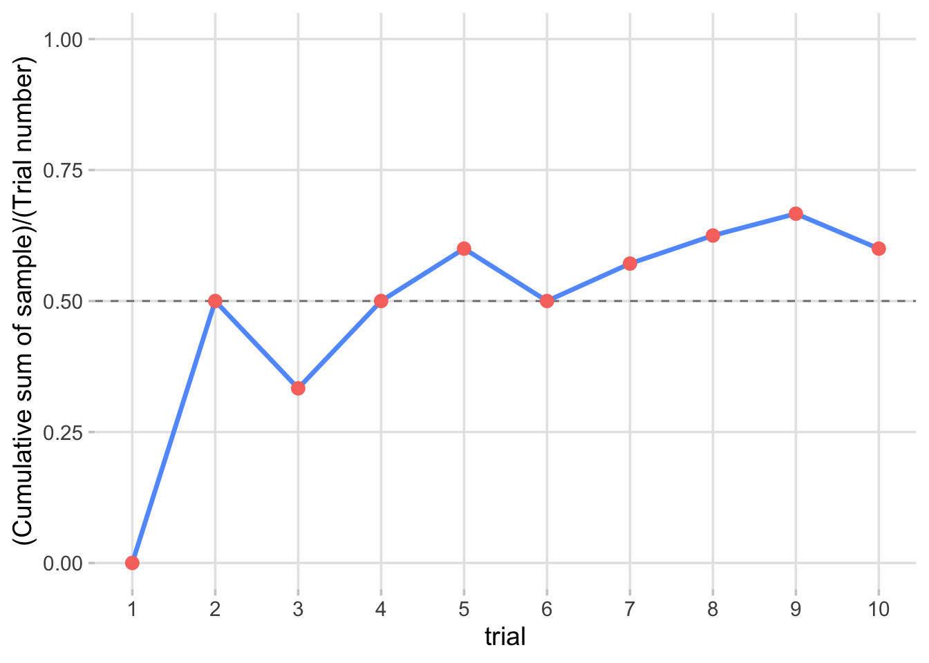
Figure 4.5: Simulation of running sample mean of Bernoulli \(p = 0.5\) trials over time
R Simulation Code (Single Sample Path):
Example 4.2
n = 10
trial = seq(1, n, by = 1)
sample = rbinom(n, 1, 1/2)

plot(trial, cumsum(sample)/trial, type = "l", ylim = c(0,1), col = "blue")
points(trial, cumsum(sample)/trial, col = "red")
abline(h = 0.5, lty = 2, col = "black")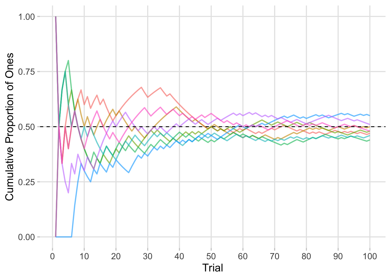
Figure 4.6: A Simulation of 20 running sample means of Bernoulli \(p = 0.5\) trials converging over 100 trials
R Simulation Code (Multiple Sample Paths):
Example 4.3
n = 100
trial = seq(1, 100, by = 1)

sample1 = rbinom(n, 1, 1/2)
sample2 = rbinom(n, 1, 1/2)
sample3 = rbinom(n, 1, 1/2)
sample4 = rbinom(n, 1, 1/2)
sample5 = rbinom(n, 1, 1/2)
sample6 = rbinom(n, 1, 1/2)
sample7 = rbinom(n, 1, 1/2)
sample8 = rbinom(n, 1, 1/2)

colors = rainbow(8)


plot(trial, cumsum(sample1)/trial, type = "l", col = colors[1], ylim = c(0,1))
lines(trial, cumsum(sample2)/trial, col = colors[2])
lines(trial, cumsum(sample3)/trial, col = colors[3])
lines(trial, cumsum(sample4)/trial, col = colors[4])
lines(trial, cumsum(sample5)/trial, col = colors[5])
lines(trial, cumsum(sample6)/trial, col = colors[6])
lines(trial, cumsum(sample7)/trial, col = colors[7])
lines(trial, cumsum(sample8)/trial, col = colors[8])
abline(h = 0.5, lty = 2, col = "black")
Empirical Probability Insight
The Law of Large Numbers gives us empirical probabilities. Consider tossing a fair coin. Define the random variable \(X\) as:
\[X = \begin{cases} 1 & \text{heads up} \\ 0 & \text{tails up} \end{cases}\]
Then as we sample more and more values of \(X\), the sample mean \(\bar{X}_n\) converges in probability to \(P(\text{heads up})\), that is:
\[\bar{X}_n \overset{p}{\longrightarrow} P(\text{heads up}).\]