Chapter 2 An Introduction to R

2.1 The Statistical Computing Language

R is used for data manipulation, statistics, and graphics. It supports a wide range of operations (+, -, <, etc.), which are used to perform calculations on vectors, arrays, and matrices. R also includes a huge collection of built-in functions, tools for generating high-quality graphs, and a wide array of user-contributed packages (organized into sets of related functions called libraries).

R can interface with procedures written in C, C++, FORTRAN, and other languages, making it extensible for advanced users. It is open-source and freely available from CRAN (The Comprehensive R Archive Network), and has seen a rapid rise in popularity in recent years.

Unlike point-and-click software tools, R allows users to write scripts that document each step of their analysis. This promotes reproducibility, version control, and transparency — all of which are essential in modern data science and academic research. With R, analyses can be automated, customized, and repeated on new datasets with minimal effort.

2.2 Installing R and RStudio

Before we can begin working with R code, we need to install both the R programming language itself and an interface to work in — such as RStudio.

2.2.1 Installing R

To install R, follow the steps below:

Visit the official R project website: https://cran.r-project.org

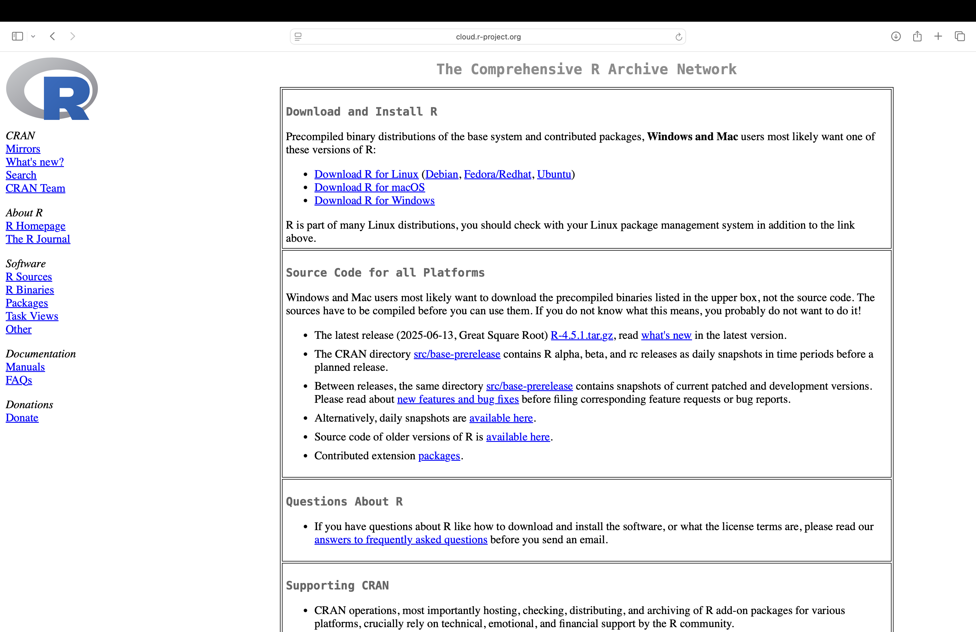
Figure 2.1: A screenshot from official R project website (You will see this page after clicking the link from step 1).

Choose your operating system:
- Windows: Click “Download R for Windows” → then “base” → then click the .exe installer link.
- macOS: Click “Download R for macOS” and choose the .pkg file appropriate for your version.
- Linux: Click “Download R for Linux” and follow distribution-specific instructions.
Run the downloaded installer and proceed with the default installation settings.

Once installed, R can be accessed directly from a terminal or used through an IDE like RStudio.

2.2.2 Installing RStudio

RStudio is a popular integrated development environment (IDE) designed specifically for R. It provides a user-friendly interface that includes:

A script editor
An R console
An environment viewer
A file browser
A plots pane and help tab

RStudio simplifies the workflow of writing and testing code, inspecting data, and generating reports.

To install RStudio:

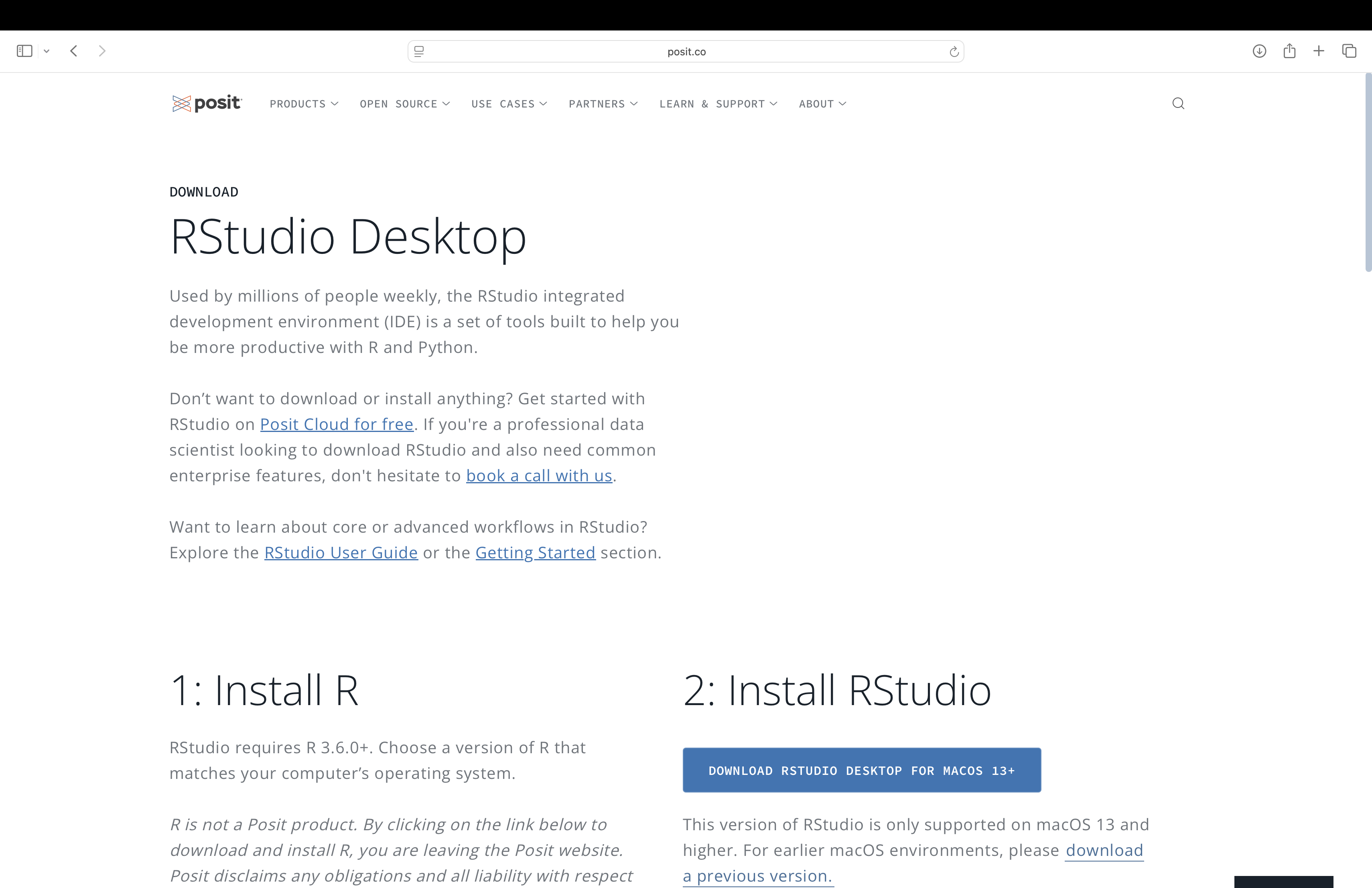
Go to https://posit.co/download/RStudio-desktop

Figure 2.2: A screenshot from RStudio Desktop download page.

Download the free version of RStudio Desktop for your operating system.
Run the installer. Once launched, RStudio will automatically detect your R installation.
Finally, you will see the following homepage when you open RStudio:

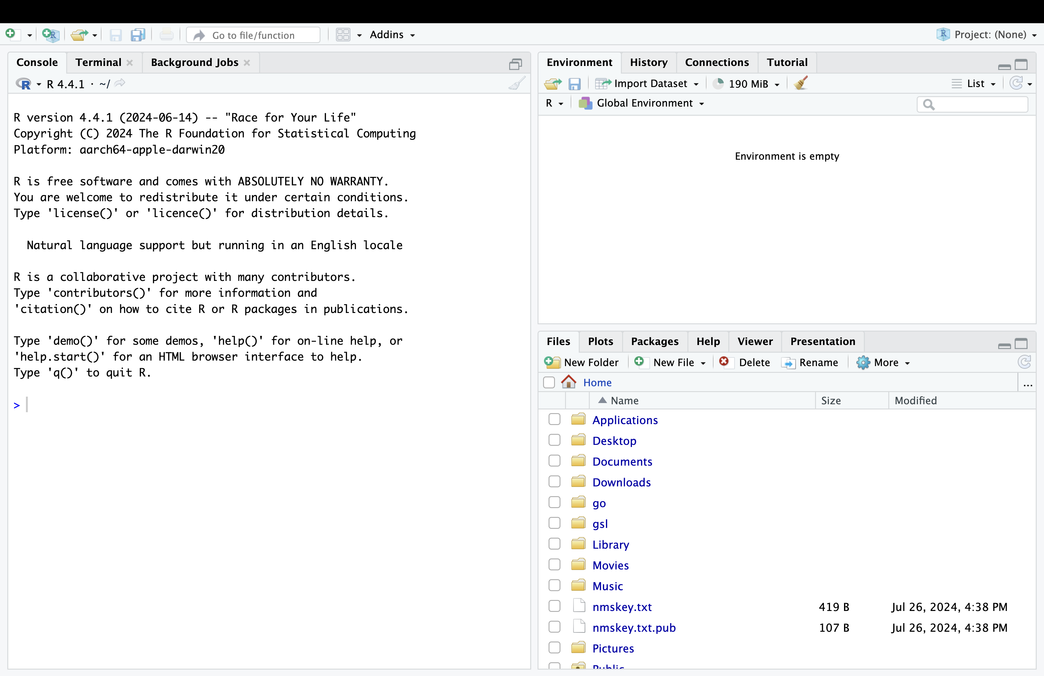
Figure 2.3: The RStudio integrated development environment.

5. To open a new script for coding, click on File → New File → R Script.

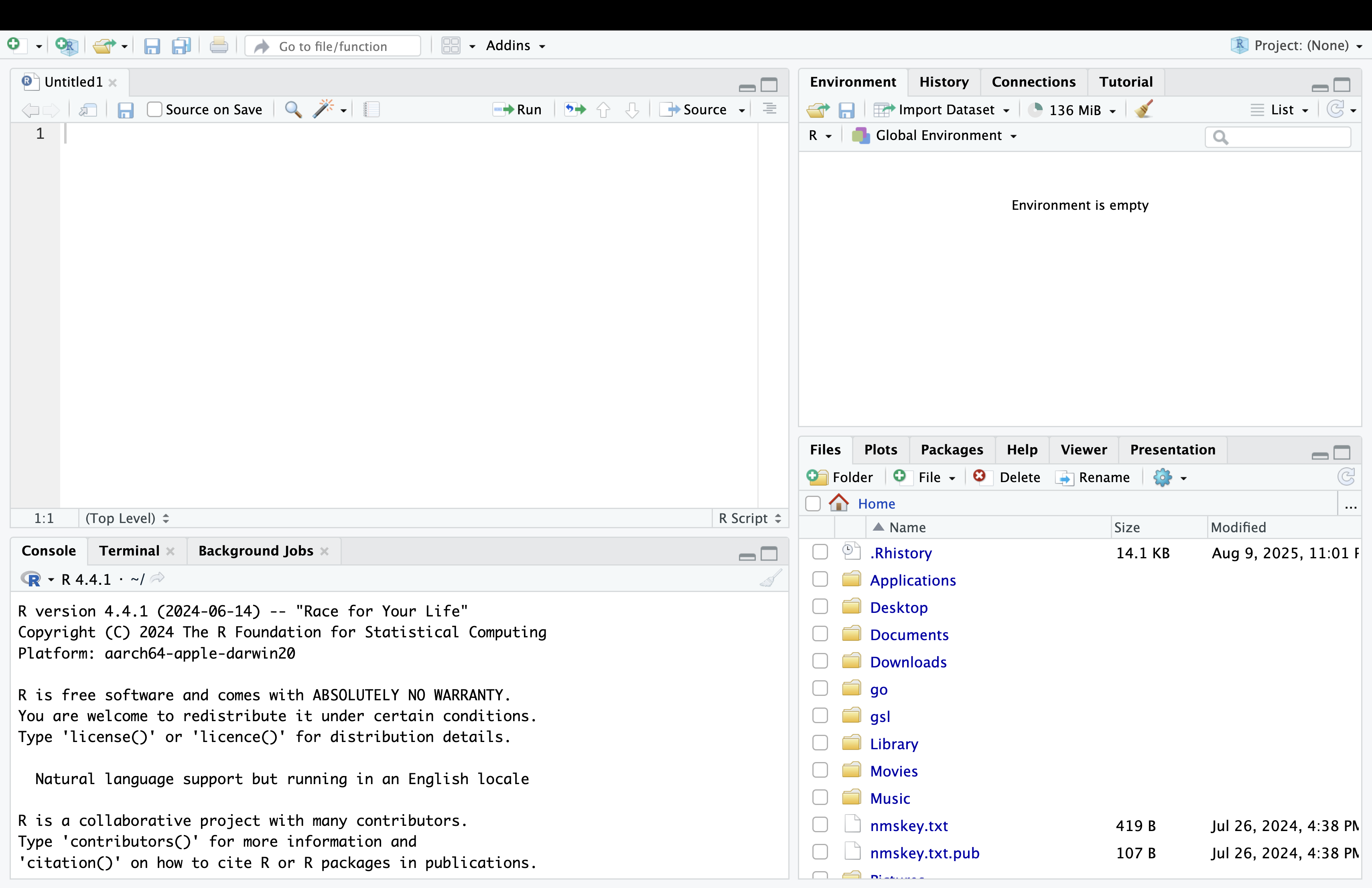
Figure 2.4: The RStudio integrated development environment with a new script.

After opening a new script, you should now see 4 main panes in the RStudio Desktop, with each serving pane serving specific purpose for coding, managing files, and viewing results:

Source Pane (Top-Left): This is where you write and edit your R scripts, R Markdown files, and other code documents. You can have multiple scripts open in tabs, making it easy to switch between different files while working on projects.
Console Pane (Bottom-Left):This is where R executes your commands directly. You can type code line-by-line here to see immediate results or view the output of scripts you run from the Source Pane. It also displays messages, errors, and warnings generated by R.
Environment/History Pane (Top-Right): The Environment tab lists all the objects (variables, data frames, functions) currently stored in your R session. The History tab records the commands you’ve executed, allowing you to review or reuse them later.
Files/Plots/Packages/Help/Viewer Pane (Bottom-Right):

Files: Browse your working directory and open files directly from here.

Plots: View visualizations generated by your code.

Packages: Manage installed R packages, load or unload them.

Help: Access R documentation and function references.

Viewer: Display web content, such as HTML outputs from R Markdown or Shiny apps.

2.2.3 Positron

RStudio is now maintained by Posit, a company that also supports tools like Shiny, Quarto, and R Markdown.

Posit also develops Positron, which is a cross-platform desktop integrated development environment (IDE) developed by Posit PBC (formerly RStudio). Built on the Visual Studio Code architecture and powered by Electron, it runs as a standalone application on Windows, macOS, and Linux. Positron is designed specifically for data science and statistical computing in R and Python, with additional support for languages such as JavaScript and Quarto documents. While not required for this course, Positron may become relevant in future workflows involving collaborative or browser-based coding.

Positron can be downloaded at https://positron.posit.co.

After completing this setup, you’re ready to begin writing and executing R code using RStudio.

2.3 An Introduction to programming in R

People use R for programming because it is specifically designed for data analysis, statistics, and visualization. It offers a rich ecosystem of packages and built-in functions that make complex statistical tasks straightforward. R is especially popular in academia and research due to its open-source nature, strong support for reproducible reporting, and seamless integration with tools like R Markdown and Shiny. Its syntax is well-suited for working with data, making it a powerful and efficient language for data scientists, statisticians, and researchers.

2.3.1 R as a Powerful Calculator

R is a powerful language for numerical and statistical computing, and it supports a wide range of mathematical operations out of the box. You can perform basic arithmetic such as addition, subtraction, multiplication, and division, as well as more advanced operations like exponentiation, logarithms, and trigonometric functions. These operations work seamlessly with individual numbers, vectors, and matrices. R also provides built-in functions to compute summary statistics like mean, standard deviation, and variance, making it ideal for data analysis and scientific computing. In the following section, we will explore how to use these operations with simple examples.

Firstly, let’s begin with basic arithmetic:

2 + 3, addition → 5;

4 - 1, subtraction → 3;

6 * 2, multiplication → 12;

8 / 2, division → 4;

5^2, exponentiation → 25;

9 %% 4, modulo (remainder) → 1;

9 %/% 4, integer division → 2.

Then, it’s going to be vector operations:

x <- c(1, 2, 3), assigning a vector variable on x;

y <- c(4, 5, 6), assigning a vector variable on y;

x + y, element-wise addition → 5 7 9;

x * y, element-wise multiplication → 4 10 18;

x^2, square each element → 1 4 9.

We are able to do math functions as well:

sqrt(16), square root → 4;

log(10), satural log → ~2.3;

log10(100), log base 10 → 2;

exp(1), e^1 → ~2.718;

abs(-5), absolute value → 5;

round(3.1415, 2), round to 2 decimals → 3.14;

sin(pi / 2) → 1;

cos(0) → 1;

tan(pi / 4) → 1.

Finally, there are some useful summery functions in R:

mean(x), average;

sum(x), total;

min(x), minimum;

max(x), maximum;

sd(x), standard deviation;

var(x), variance.

2.3.2 Basic R Data Structures

The primary data structures in R are vectors, lists, matrices, arrays, factors, and data frames.

Vectors

In R, vectors are the fundamental building blocks for data storage and manipulation. A vector is a one-dimensional sequence that contains elements of the same type, such as numbers, characters, or logical values. They are widely used in R for performing calculations, storing results, and processing data efficiently. Vectors support a variety of operations including indexing, filtering, and element-wise arithmetic, making them essential for both basic programming tasks and advanced statistical analysis. Understanding how to create and work with vectors is a crucial first step in learning R programming.

For example:

Assigning a variable be a vector
v <- c(1, 2, 3, 4, 5)

Lists

In R, a list is a flexible data structure that can store elements of different types and sizes, such as numbers, strings, vectors, or even other lists. Unlike vectors, which require all elements to be of the same type, lists allow you to group together a variety of data types in a single object. This makes lists especially useful for organizing complex or mixed data, returning multiple results from functions, and building structured objects like data frames. Understanding how to create, access, and manipulate lists is essential for working effectively with more advanced R data structures.

For example:

Creating a list contains some random elements
my_list <- list(name = "Alice", age = 25, scores = c(90, 85, 88), passed = TRUE)

Accessing code:
my_list$name         # Access by name
my_list[[2]]         # Access by index
my_list[["scores"]]  # Another way to access 'scores'

Modifying an element of the list:
my_list$age <- 26
my_list$new_field <- "Added!"

Matrices

In R, a matrix is a two-dimensional data structure that stores elements of the same type, typically numeric or logical values. Matrices are widely used in mathematical computations, especially in linear algebra, statistics, and data analysis. They are essentially vectors with a specified number of rows and columns, and support a wide range of operations such as addition, multiplication, transposition, and inversion. R provides straightforward functions to create, access, and manipulate matrices, making them a fundamental tool for performing structured data analysis and mathematical modeling.

For example:

# Create a 3x2 matrix filled by column (default)
m <- matrix(c(1, 2, 3, 4, 5, 6), nrow = 3, ncol = 2)

Accessing elements in the matrix above:
m[1, 2]     # Element in row 1, column 2
m[ , 1]     # All rows of column 1
m[2, ]      # All columns of row 2

Basic matrices operations:
t(m)        # Transpose
m %*% t(m)  # Matrix multiplication
det(m)      # Determinant (square matrix only)
solve(m)    # Inverse (if square and invertible)

Arrays

In R, an array is a multi-dimensional data structure that stores elements of the same type, such as numeric or logical values. Unlike matrices, which are limited to two dimensions, arrays can have two or more dimensions, making them suitable for representing more complex data like multiple matrices or higher-dimensional datasets. Arrays are useful in simulations, image processing, and situations where data varies across multiple levels, such as time, location, or category. Understanding how to create and work with arrays allows you to efficiently manage and analyze structured data in higher dimensions.

For example:

# Create a 3D array (2 rows × 3 columns × 2 layers)
a <- array(1:12, dim = c(2, 3, 2))

Accessing elements in the array above:
a[1, 2, 1]     # Element at row 1, column 2, layer 1
a[ , , 2]      # All rows and columns in layer 2

Factors

In R, a factor is a data structure used to represent categorical variables, such as labels or groupings. Unlike regular character vectors, factors store both the unique values (called levels) and their underlying integer codes, making them more efficient and meaningful for statistical modeling and data analysis. Factors are especially useful when working with data that falls into fixed categories, like gender, education level, or survey responses. They are automatically treated as categorical variables in functions like linear models, making them an essential tool in R for handling qualitative data.

For example:

Creating a factor
gender <- factor(c("Male", "Female", "Female", "Male"))

Check levels
levels(gender)
# [1] "Female" "Male"

Data Frames

In R, a data frame is a fundamental data structure used for storing tabular data. It organizes data into rows and columns, where each column can hold a different type of variable—such as numbers, strings, or logical values—but all columns must have the same number of rows. Data frames are ideal for handling datasets in statistical analysis, machine learning, and data visualization. They closely resemble tables in spreadsheets or databases, making them intuitive and practical for real-world data manipulation. Mastering data frames is essential for effective data analysis in R.

For example:

Creating a data frame:
df <- data.frame(name = c("Alice", "Bob", "Charlie"), age = c(25, 30, 28), passed = c(TRUE, FALSE, TRUE))

Accessing data from the data frame above:
df$name        # Access 'name' column
df[1, ]        # First row
df[ ,2]        # Second column
df[2, 3]       # Row 2, column 3

Adding a new column or row:
df$score <- c(90, 85, 88)  # Add new column
df <- rbind(df, data.frame(name="David", age=27, passed=TRUE, score=92))  # Add new row

Some useful functions:
str(df)        # Structure of the data frame
summary(df)    # Summary stats
nrow(df)       # Number of rows
ncol(df)       # Number of columns

2.3.3 Using Basic Functions in R

R provides many built-in functions that allow you to perform calculations, transformations, or extract summary statistics from data. Here are some commonly used basic functions:

x <- c(10, 3, 8, 25, 7)

# Find the maximum and minimum values
max(x)
min(x)

# Sort the vector
sort(x)     # ascending order
sort(x, decreasing = TRUE)  # descending order

# Find the order (ranks) of elements
order(x)

These functions work on vectors, and many of them are also applicable to data frames or matrices when used with additional arguments.

2.3.4 Make a Histogram Using RStudio

We will use the faithful dataset, which is included with R. It contains two numeric variables. For this demonstration, we will generate a histogram of one of those variables.

Follow the steps below:

First, decide which dataset you want to use. In this case, we use the built-in faithful dataset.
To view the variable names in any dataset, use the names() function. This will display all available columns:

# Display variable names in the dataset
names(faithful)

To create a histogram of one variable:

# Create a basic histogram
hist(faithful$waiting)

This will produce a simple histogram showing the distribution of values in the selected column.

You can also access the numeric components of the histogram using the plot = FALSE argument. This prevents the histogram from being drawn and instead returns a list of values used in the plot:

# View the histogram breakpoints
hist(faithful$waiting, plot = FALSE)$breaks

# View the counts in each interval
hist(faithful$waiting, plot = FALSE)$counts

These functions return numeric vectors. The first shows where each interval begins and ends, and the second shows how many values fall within each interval.

Example output:

[1]  40  45  50  55  60  65  70  75  80  85  90  95 100
[1]   4  22  33  24  14  10  27  54  55  23   5   1

These tools allow you to not only create visual summaries, but also work with the underlying values programmatically — which is useful for analysis, customization, or reporting.

2.3.5 Installing and Loading Packages

R has a large ecosystem of additional packages that provide specialized functions. Before you can use a package, you typically need to:

Install the package (only once):

install.packages("ggplot2")

Load the package into your R session:

library(ggplot2)

Once loaded, you can use functions from that package — for example, ggplot() from the ggplot2 package.

Tip: You only need to install a package once, but you must load it with library() every time you restart RStudio.

You can search for packages or view installed ones using:

# View all installed packages
installed.packages()

# Search for packages by keyword
help.search("regression")

R packages are stored in CRAN (Comprehensive R Archive Network), which you accessed when installing R. There are also GitHub-hosted packages for advanced users.