Chapter 8 Analysis of Variance
ANOVA (Analysis of Variance) is used to compare multiple means.
Suppose we have \(k\) groups \((k \geqslant 3)\) and each group is given a treatment.
The ANOVA model is:
\[ Y_{ij} = \mu + \tau_i + \varepsilon_{ij}, \quad \varepsilon_{ij} \sim N(0, \sigma^2) \]
Where:
- \(Y_{ij}\): outcome on unit \(j\) in group \(i\)
- \(\mu\): overall mean
- \(\tau_i\): treatment-specific effect for group \(i\)
- \(\varepsilon_{ij}\): error term, assumed normally distributed
- \(\mu_i = \mu + \tau_i\): group mean
The equivalent form of the ANOVA model is:
\[ Y_{ij} = \mu_i + \varepsilon_{ij}, \quad \varepsilon_{ij} \sim \mathcal{N}(0, \sigma^2) \]
\[ \begin{array}{c|c|c|c|c} \text{Group 1} & \text{Group 2} & \cdots & \text{Group } K \\ \hline X_{11} & X_{21} & \cdots & X_{K1} \\ X_{12} & X_{22} & \cdots & X_{K2} \\ \vdots & \vdots & \ddots & \vdots \\ X_{1n_1} & X_{2n_2} & \cdots & X_{Kn_K} \\ \hline \bar{X}_1 & \bar{X}_2 & \cdots & \bar{X}_K \\ S_1^2 & S_2^2 & \cdots & S_K^2 \\ n_1 & n_2 & \cdots & n_K \\ \end{array} \]
Where:
- \(\bar{X}_i\): sample mean of group \(i\)
- \(S_i^2\): sample variance of group \(i\)
- \(n_i\): sample size of group \(i\)
Total Sample Size and Overall Mean
Total sample size:
\[ n = n_1 + n_2 + \cdots + n_k \]
Overall sample mean:
\[ \bar{X} = \frac{1}{n} \sum_{i=1}^k \sum_{j=1}^{n_i} X_{ij} = \frac{1}{n} \sum_{i=1}^k n_i \bar{X}_i \]
Sources of Variation
Variation within groups (SSW / SSE):
\[ \text{SSE} = \sum_{i=1}^k (n_i - 1) \cdot S_i^2 \]
This represents error or residual variation.
Variation between groups (SSB / SSTr):
\[ \text{SSTr} = \sum_{i=1}^k n_i \cdot (\bar{X}_i - \bar{X})^2 \]
This captures the treatment effect (how group means differ from overall mean).
Total Variation
\[ \text{SSTotal} = \sum_{i=1}^k \sum_{j=1}^{n_i} (X_{ij} - \bar{X})^2 \]
Decomposition Identity
\[ \text{SSTotal} = \text{SSTr} + \text{SSE} \]
ANOVA Table
| Source | df | SS | MS | F-Statistic |
|---|---|---|---|---|
| Treatment | k - 1 | SSTr | MSTr = SSTr / (k - 1) | F* = MSTr / MSE |
| Error | n - k | SSE | MSE = SSE / (n - k) | |
| Total | n - 1 | SSTotal |
Where \(MS = \dfrac{SS}{df}\)
Hypothesis Test \[ \begin{aligned} H_0\!: &\quad \mu_1 = \mu_2 = \cdots = \mu_k \\ &\quad \text{(all means are equal → all treatments equally effective)} \\ \\ H_a\!: &\quad \text{At least one } \mu_j \text{ (for } j = 1, \dots, k\text{) is different} \\ &\quad \text{(→ at least one treatment has a different effect)} \end{aligned} \]
Test Statistic
\[ F^* = \frac{\text{MSTr}}{\text{MSE}} = \frac{\text{SSTr} / (k - 1)}{\text{SSE} / (n - k)} \sim F_{(k - 1,\ n - k)} \]
Reference Distribution
The test statistic follows an \(F\)-distribution with:
- numerator degrees of freedom = \(k - 1\)
- denominator degrees of freedom = \(n - k\)
P-value
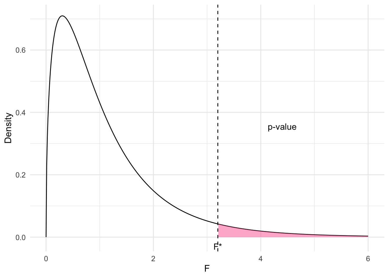
Figure 8.1: F-distribution with shaded p-value area
The Data Matrix
The following table shows last year’s sales data for a small business. The sample is put into a matrix format in which each of the three columns corresponds to one of the three countries in which the company does business. The numbers in the cell represent the sales (in units of \(\$ 1000\) ) made in that country last year. These data will be used to develop the theory underlying Analysis of Variance, or, for short, ANOVA.
| Country A | Country B | Country C | |
|---|---|---|---|
| 6 | 10 | 14 | |
| 10 | 8 | 13 | |
| 7 | 12 | 11 | |
| 9 | 10 | 10 | |
| Average | 8 | 10 | 12 |
Altogether, there were 12 sales last year that totaled $120 – so the average sale was $10.
The column (country) averages are:
Column 1 (Country A): $8
Column 2 (Country B): $10
Column 3 (Country C): $12
Now we will begin our study of how to make a statistically valid prediction of the next sales figure. In that regard, there are two possible situations that can occur:
- The country of the next sale (observation) is not known.
- The country of the next sale is known.
Situation 1.
Without any additional information, the best prediction is the sample mean \(\$ 10\). This prediction is best in the least squares sense - that is, if \(\$ 10\) had been used to predict each of the 12 observations in the sample, then the total of the squared errors \(S S_{\text {Total }}\) would be as small as possible. In our data set, \(S S_{\text {Total }}\) equals 60 . That figure can be verified by calculating \(\sum\left(x_{i}-10\right)^{2}\) for each observation \(x_{i}\) of the sample.
Situation 2. One-factor ANOVA Model.
If the country of the next sale is known, then two different predictions are possible for the next sales figure:
- The sample mean \(\$ 10\).
- The mean of the sales of the country in which the next sale will occur. (In this case, \(\$ 8\) if the next sale will occur in Country A, \(\$ 10\) in Country B, or \(\$ 12\) in Country C.) This prediction ignores the information present in the sales figures from the other two countries.
The Null Hypothesis for One-Factor ANOVA
We have discussed the prediction possibilities for one-factor ANOVA models. Now, we will learn how to test the statistical significance of a one-factor ANOVA model. Let’s suppose that we want to predict the next sales figure, and that we know the country in which this sale will occur. Without any statistical testing, we can always by default use the sample mean \(\$ 10\) to predict the next sale. The default prediction, the sample mean, doesn’t use any information about the country (column) in which the sale will occur.
However, if instead we use the mean of the observations in only one column (the column that corresponds to the particular country in which we know the next sale will occur), then we have to test the null hypothesis
\[ H_{0}: \mu_{C O L 1}, \mu_{C O L 2}, \mu_{C O L 3}, \text { are equal } \]
and reject it in favor of the alternative hypothesis
\[ H_{a}: \mu_{C O L 1}, \mu_{C O L 2}, \mu_{C O L 3}, \text { are NOT all equal } \]
If the null hypothesis is rejected, then we can be statistically confident that the column means are not all equal, and therefore that the individual column means (i. e., \(\$ 8, \$ 10, \$ 12\) ) can be used to predict the amount of the next sale. If the next sale was going to occur in Country A , then the prediction would be \(\$ 8\). If the next sale was going to occur in Country B, then the prediction would be \(\$ 10\). If the next sale was going to occur in Country C , then the prediction would be \(\$ 12\).
The One-Factor ANOVA F Test
To test the null hypothesis stated above, we have to calculate an F-statistic. If \(F_{*}>F_{(c-1, n-c), \alpha}\), then reject \(H_{0}\), and use the sample column means to predict future observations. Otherwise, do not reject \(H_{0}\) and use the overall sample mean to predict future observations.
ANOVA Table
To see how this \(F_{*}\) is calculated, see the ANOVA Table below.
| Source of Variation |
Degrees of Freedom \((\mathrm{df})\) |
Sum of Square \((\mathrm{SS})\) |
Mean Sum of Squares \((\) MSS \()\) |
F Ratio |
|---|---|---|---|---|
| Treatments | \(\mathrm{c}-1\) | SST | \(\frac{\text { SST }}{c-1}\) | \(F=\frac{\text { MST }}{\text { MSE }}\) |
| Error | \(\mathrm{n}-\mathrm{c}\) | SSE | \(\frac{\text { SSE }}{n-c}\) | |
| Total | \(\mathrm{n}-1\) | \(\mathrm{SS}_{\mathrm{Total}}\) | ||
Calculation of \(\mathrm{SS}_{\mathrm{Total}}\)
If no model is used, then the predictions for each of the 12 observations will be 10 . If these predictions are used, the squared error of these 12 predictions is given in the table below.
| Country A | Country B | Country C |
|---|---|---|
| 16 | 0 | 16 |
| 0 | 4 | 9 |
| 9 | 4 | 1 |
| 1 | 0 | 0 |
Prediction Errors Squared when NO Factor is used \((\) Total \()=60\).
Calculation of SSE
If the column model is used, then the 12 observations would have the following 12 predictions, where \(\$ 8\) is the average for the first column, \(\$ 10\) is the average for the second column, and \(\$ 12\) is the average for the third column.
| Country A | Country B | Country C |
|---|---|---|
| 8 | 10 | 12 |
| 8 | 10 | 12 |
| 8 | 10 | 12 |
| 8 | 10 | 12 |
Calculation of SSE
Using the above 12 predictions, the errors squared are shown in the table below.
| Country A | Country B | Country C |
|---|---|---|
| 4 | 0 | 4 |
| 4 | 4 | 1 |
| 1 | 4 | 1 |
| 1 | 0 | 4 |
Errors Squared when the Column Factor is used \((\) Total \()=28\).
Calculation of SST
The units explained by the column model are calculated by finding the square of each prediction change when moving from NO model to the column model. The following table presents the square of each prediction change:
| Country A | Country B | Country C |
|---|---|---|
| 4 | 0 | 4 |
| 4 | 0 | 4 |
| 4 | 0 | 4 |
| 4 | 0 | 4 |
Table of the Square of the Prediction Change when Moving from NO Model to the Column Model \((\) Total \()=32\).
ANOVA Table
The ANOVA Table for the column factor can now be filled in as shown below:
| Source of Variation |
Degrees of Freedom \((\mathrm{df})\) |
Sum of Square \((\mathrm{SS})\) |
Mean Sum of Squares \((\) MSS \()\) |
F Ratio |
|---|---|---|---|---|
| Treatments | 2 | 32 | \(\frac{32}{2}=16\) | \(\frac{16}{3.1111}=5.1428\) |
| Error | 9 | 28 | \(\frac{28}{9}=3.1111\) | |
| Total | 11 | 60 |
So for this one-factor ANOVA model, \(F_{*}=5.1428\).
Conclusion
If the null hypothesis is true, then the F-statistic should be a value from the \(F_{2,9}\) distribution. Referring to the table that contains the upper 0.05 cut-off points of F distributions, we see that \(F_{(2,9), 0.05}=4.256\). Since 5.1428 is greater than 4.256 , this tells us that the F -statistic is in the upper 0.05 of the \(F_{2,9}\) distribution. Therefore we reject the null hypothesis at the 0.05 significance level, and we conclude that the country means are not all the same. Thus, the prediction for the next sale in a known country is the mean of all the previous sales in that country.
# R Code;
salesA=c(6,10,7,9);
salesB=c (10, 8,12,10);
salesC=c(14,13,11,10);
sales=c(salesA,salesB,salesC);
country=c(rep(1,4),rep(2,4),rep(3,4));
oneway.test(sales~country,var.equal=TRUE);
##
## One-way analysis of means
##
## data: sales and country
## F = 5.1429, num df = 2, denom df = 9, p-value =
## 0.0324# R Code;
# Another way: using lm;
salesA=c(6,10,7,9);
salesB=c (10, 8,12,10);
salesC=c(14,13,11,10);
sales=c(salesA,salesB,salesC);
country=c(rep(1,4),rep(2,4),rep(3,4));
anova(lm(sales~factor(country)));## Analysis of Variance Table
##
## Response: sales
## Df Sum Sq Mean Sq F value Pr(>F)
## factor(country) 2 32 16.0000 5.1429 0.0324 *
## Residuals 9 28 3.1111
## ---
## Signif. codes:
## 0 '***' 0.001 '**' 0.01 '*' 0.05 '.' 0.1 ' ' 1Officially, to use the predictions from an ANOVA model, three assumptions about the populations from which the sample was taken must be satisfied:
- Each population has a Normal distribution.
- Each population has the same standard deviation \(\sigma\).
- The observations are mutually independent of one another.
Formulas
Sum of Squares for Treatments (a.k.a. between-treatments variation or Explained)
\[ S S T=\sum_{j=1}^{k} n_{j}\left(\bar{x}_{j}-\overline{\bar{x}}\right)^{2} \]
Sum of Squares for Error (a.k.a. within-treatments variation or Unexplained)
\[ S S E=\sum_{j=1}^{k} \sum_{i=1}^{n_{j}}\left(x_{i j}-\bar{x}_{j}\right)^{2}=\left(n_{1}-1\right) s_{1}^{2}+\ldots+\left(n_{k}-1\right) s_{k}^{2} \]
Mean Square for Treatments
\[ M S T=\frac{S S T}{k-1} \]
Mean Square for Error
\[ M S E=\frac{S S E}{n-k} \]
Test Statistic
\[ F=\frac{M S T}{M S E} \]
Exercise
A statistics practitioner calculated the following statistics:
\[ \begin{array}{|c|c|c|c|} \hline \textbf{Statistic} & \textbf{1} & \textbf{2} & \textbf{3} \\ \hline n & 5 & 5 & 5 \\ \hline \bar{x} & 10 & 15 & 20 \\ \hline s^2 & 50 & 50 & 50 \\ \hline \end{array} \]
Complete the ANOVA table.
Solution
\[ \begin{aligned} & \overline{\bar{x}}=\frac{5(10)+5(15)+5(20)}{5+5+5}=15 \\ & S S T=5(10-15)^{2}+5(15-15)^{2}+5(20-15)^{2}=250 \\ & S S E=(5-1)(50)+(5-1)(50)+(5-1)(50)=600 \end{aligned} \]
ANOVA Table
| Source of Variation | Degrees of Freedom (df) | Sum of Square (SS) | Mean Sum of Squares (MSS) | F Ratio |
|---|---|---|---|---|
| Treatments | 2 | 250 | \(\frac{250}{2}=125\) | \(\frac{125}{50}=2.50\) |
| Error | 12 | 600 | \(\frac{600}{12}=50\) | |
| Total | 14 | 850 |
Exercise
A statistics practitioner calculated the following statistics:
\[ \begin{array}{|c|c|c|c|} \hline \textbf{Statistic} & \textbf{1} & \textbf{2} & \textbf{3} \\ \hline n & 4 & 4 & 4 \\ \hline \bar{x} & 20 & 22 & 25 \\ \hline s^2 & 10 & 10 & 10 \\ \hline \end{array} \]
Complete the ANOVA table.
Solution
\[ \begin{aligned} & \overline{\bar{x}}=\frac{4(20)+4(22)+4(25)}{4+4+4}=22.33 \\ & S S T=4(20-22.33)^{2}+4(22-22.33)^{2}+4(25-22.33)^{2}=50.67 \\ & S S E=(4-1)(10)+(4-1)(10)+(4-1)(10)=90 \end{aligned} \]
ANOVA Table
| Source of Variation | Degrees of Freedom (df) | Sum of Square (SS) | Mean Sum of Squares (MSS) | F Ratio |
|---|---|---|---|---|
| Treatments | 2 | 50.67 | \(\frac{50.67}{2}=25.33\) | \(\frac{25.33}{10}=2.53\) |
| Error | 9 | 90 | \(\frac{90}{9}=10\) | |
| Total | 11 | 140.67 |
Exercise
A consumer organization was concerned about the differences between the advertised sizes of containers and the actual amount of product. In a preliminary study, six packages of three different brands of margarine that are supposed to contain 500 ml were measured. The differences from 500 ml are listed here. Do these data provide sufficient evidence to conclude that differences exist between the three brands? Use \(\alpha=0.05\).
| Brand 1 | Brand 2 | Brand 3 |
|---|---|---|
| 1 | 2 | 1 |
| 3 | 2 | 2 |
| 3 | 4 | 4 |
| 0 | 3 | 2 |
| 1 | 0 | 3 |
| 0 | 4 | 4 |
Exercise on 3 bounds
Consider
\(\alpha = 0.05\)
| Brand 1 | Brand 2 | Brand 3 |
|---|---|---|
| \(x_{11}=1\) | \(x_{21}=2\) | \(x_{31}=1\) |
| \(x_{12}=3\) | \(x_{22}=2\) | \(x_{32}=2\) |
| 3 | 4 | 4 |
| 0 | 3 | 2 |
| 1 | 0 | 3 |
| \(x_{16}=0\) | \(x_{26}=4\) | \(x_{36}=4\) |
| \(n_1=6\) | \(n_2=6\) | \(n_3=6\) |
Overall Sample Size
\[ n = n_1 + n_2 + n_3 = 18 \]
Sample Means
Group 1: \[ \bar{X}_1 = \frac{1}{n_1} \sum_{j=1}^{n_1} x_{1j} = \frac{1}{6}(1 + 3 + \dots + 0) = 1.33 \]
Group 2: \[ \bar{X}_2 = \frac{1}{n_2} \sum_{j=1}^{n_2} x_{2j} = \frac{1}{6}(2 + 2 + \dots + 4) = 2.50 \]
Group 3: \[ \bar{X}_3 = \frac{1}{n_3} \sum_{j=1}^{n_3} x_{3j} = \frac{1}{6}(1 + 2 + \dots + 4) = 2.67 \]
Overall Mean
\[ \bar{X} = \frac{1}{n} \sum_{i=1}^{k} \sum_{j=1}^{n_i} x_{ij} = \frac{1 + 3 + \dots + 0 + 2 + 2 + \dots + 4 + 1 + 2 + \dots + 4}{18} \]
\[ = \frac{1}{n} \sum_{i=1}^{k} n_i \bar{X}_i = \frac{1}{18} \left[ (6)(1.33) + (6)(2.5) + (6)(2.67) \right] \]
\[ = 2.17 \]
| Brand 1 | Brand 2 | Brand 3 |
|---|---|---|
| \(x_{11} = 1\) | \(x_{21} = 2\) | \(x_{31} = 1\) |
| \(x_{12} = 3\) | \(x_{22} = 2\) | \(x_{32} = 2\) |
| 3 | 4 | 4 |
| 0 | 3 | 2 |
| 1 | 0 | 3 |
| \(x_{16} = 0\) | \(x_{26} = 4\) | \(x_{36} = 4\) |
| \(n_1 = 6\) | \(n_2 = 6\) | \(n_3 = 6\) |
| \(\bar{x}_1 = 1.33\) | \(\bar{x}_2 = 2.50\) | \(\bar{x}_3 = 2.67\) |
Sample Variances
Group 1:
\[ S_1^2 = \frac{1}{n_1 - 1} \sum_{j=1}^{n_1} (x_{1j} - \bar{x}_1)^2 \]
\[ = \frac{1}{6 - 1} \left[ (1 - 1.33)^2 + \dots + (0 - 1.33)^2 \right] \]
\[ = 1.87 \]
Group 2:
\[ S_2^2 = \dots = 2.30 \]
Group 3:
\[ S_3^2 = \dots = 1.47 \]
| Brand 1 | Brand 2 | Brand 3 |
|---|---|---|
| \(x_{11} = 1\) | \(x_{21} = 2\) | \(x_{31} = 1\) |
| \(x_{12} = 3\) | \(x_{22} = 2\) | \(x_{32} = 2\) |
| 3 | 4 | 4 |
| 0 | 3 | 2 |
| 1 | 0 | 3 |
| \(x_{16} = 0\) | \(x_{26} = 4\) | \(x_{36} = 4\) |
| \(n_1 = 6\) | \(n_2 = 6\) | \(n_3 = 6\) |
| \(\bar{x}_1 = 1.33\) | \(\bar{x}_2 = 2.50\) | \(\bar{x}_3 = 2.67\) |
| \(S_1^2 = 1.87\) | \(S_2^2 = 2.30\) | \(S_3^2 = 1.47\) |
Overall mean:
\[
\bar{x} = 2.17, \quad n = 18
\]
Within (Error)
\[ SSE = \sum_{i=1}^{3} (n_i - 1) S_i^2 = (6 - 1)(1.87) + (6 - 1)(2.30) + (6 - 1)(1.47) \]
\[ = \boxed{28.20} \]
Between (Treatment effect)
\[ SS_{\text{Tot}} = \sum_{i=1}^{3} n_i (\bar{x}_i - \bar{x})^2 = 6(1.33 - 2.17)^2 + 6(2.50 - 2.17)^2 + 6(2.67 - 2.17)^2 \]
\[ = \boxed{6.39} \]
ANOVA Table
\[ MS = \frac{SS}{df} \]
| Source of Variation | Degrees of Freedom (df) | Sum of Squares (SS) | Mean Sum of Squares (MSS) | F Ratio |
|---|---|---|---|---|
| Treatment | \(3 - 1 = 2\) | 6.39 | \(\frac{6.39}{2} = 3.195\) | \(\frac{3.195}{1.88} = 1.70\) |
| Error | \(18 - 3 = 15\) | 28.20 | \(\frac{28.20}{15} = 1.88\) | |
| Total | \(18 - 1 = 17\) | 34.59 | \(\times\) |
Hypothesis Test
\[ \begin{aligned} H_0\!: &\quad \mu_1 = \mu_2 = \mu_3 \\ &\quad \text{(all means are equal} \rightarrow \text{ all treatments equally effective)} \\ \\ H_a\!: &\quad \text{At least one } \mu_j,\ j = 1, \dots, 3\ \text{ is different} \\ &\quad \text{(} \rightarrow \text{ at least one treatment has a different effect)} \end{aligned} \]
Test Statistic
\[ F^* = \frac{MS_{\text{Tr}}}{MSE} = \frac{SS_{\text{Tr}}/(k-1)}{SSE/(n-k)} = 1.70 \sim F_{(2,15)} \]
F distribution with numerator df = 2 and denominator df = 15.
\[ \text{p-value} > 0.100 > 0.05 \quad (\alpha) \]
Conclusion of ANOVA
There is insufficient evidence to reject
\[
H_0: \mu_1 = \mu_2 = \mu_3
\]
The analysis from ANOVA suggests that all 3 groups have the same mean.
What if \(H_0\) had been rejected?
Suppose we rejected \(H_0\).
Which mean (or means) are different?
\[ \mu_1,\ \mu_2,\ \mu_3 \]
Pairwise Comparisons
We would compare the means in pairs:
- \(\mu_1\) vs. \(\mu_2\)
- \(\mu_1\) vs. \(\mu_3\)
- \(\mu_2\) vs. \(\mu_3\)
Number of comparisons:
\[
\binom{k}{2}
\]
Solution
Step 1. State Hypotheses.
\(\mu_{i}=\) population mean for differences from 500 ml (brand \(i\), where \(i=1,2,3\) ).
\(H_{0}: \mu_{1}=\mu_{2}=\mu_{3}\)
\(H_{a}\) : At least two means differ.
Step 2. Compute test statistic.
| Brand 1 | Brand 2 | Brand 3 | |
|---|---|---|---|
| Mean | 1.33 | 2.50 | 2.67 |
| Variance | 1.87 | 2.30 | 1.47 |
Grand mean = \(\bar{x} = 2.17\).
\[ SST = 6(1.33 - 2.17)^2 + 6(2.50 - 2.17)^2 + 6(2.67 - 2.17)^2 = 6.387 \approx 6.39 \]
\[ SSE = (6 - 1)(1.87) + (6 - 1)(2.30) + (6 - 1)(1.47) = 28.20 \]
ANOVA Table
| Source of Variation | Degrees of Freedom (df) | Sum of Square (SS) | Mean Sum of Squares (MSS) | F Ratio |
|---|---|---|---|---|
| Treatments | 2 | 6.39 | \(\frac{6.39}{2}=3.195\) | \(\frac{3.195}{1.88}=1.70\) |
| Error | 15 | 28.20 | \(\frac{28.20}{15}=1.88\) | |
| Total | 17 | 34.59 |
Step 3. Find Rejection Region. We reject the null hypothesis only if
\[ F>F_{\alpha, k-1, n-k} \]
If we let \(\alpha=0.05\), the rejection region for this exercise is
\[ F>F_{0.05,2,15}=3.682 \]
Step 4. Conclusion.
We found the value of the test statistic to be \(F=1.70\). Since \(F=1.70<F_{0.05,2,15}=3.682\), we can’t reject \(H_{0}\). Thus, there is not evidence to infer that the average differences differ between the three brands.
# R Code;
brand1=c(1,3,3,0,1,0);
brand2=c (2,2,4,3,0,4);
brand3=c(1,2,4,2,3,4);
differences=c(brand1,brand2,brand3);
brand=c(rep(1,6),rep(2,6),rep(3,6));
oneway.test(differences~brand,var.equal=TRUE);
##
## One-way analysis of means
##
## data: differences and brand
## F = 1.6864, num df = 2, denom df = 15, p-value
## = 0.2185
##Margarine example
| Df | Sum Sq | Mean Sq | \(F\) value | |
|---|---|---|---|---|
| brand | 2 | 6.3333 | 3.1667 | 1.6864 |
| Residuals | 15 | 28.1667 | 1.8778 | 0.2185 |
Exercise
The friendly folks a the Internal Revenue Service (IRS) in the United States and Canada Revenue Agency (CRA) are always looking for ways to improve the wording and format of its tax return forms. Three new forms have been developed recently. To determine which, if any, are superior to the current form, 120 individuals were asked to participate in an experiment. Each of the three new forms and the currently used form were filled out by 30 different people. The amount of time (in minutes) taken by each person to complete the task was recorded. What conclusions can be drawn from these data?
R Code
#Step 1. Entering data;
# importing data;
# url of tax return forms;
forms_url =
"https://mcs.utm.utoronto.ca/"nosedal/data/tax-forms.txt"
forms_data= read.table(forms_url,header=TRUE);
names(forms_data);
forms_data[1:4, ];
R Code
## [1] "Form1" "Form2" "Form3" "Form4"
##   Form1 Form2 Form3 Form4
## 1    23    88   116   103
## 2    59   114   123   122
## 3    68    81    64   105
## 4   122    41   136    73
R Code
#Step 2. ANOVA;
time1=forms_data$Form1;
time2=forms_data$Form2;
time3=forms_data$Form3;
time4=forms_data$Form4;
length(forms_data$Form1);
times=c(time1,time2,time3,time4);
forms=c(rep(1,30),rep(2,30),rep(3,30),rep(4,30));
oneway.test(times~forms,var.equal=TRUE)
R Code
## [1] 30
##
## One-way analysis of means
##
## data: times and forms
## F = 2.9358, num df = 3, denom df = 116, p-value
## = 0.03632
Assumptions of ANOVA
Model
\[ Y_{ij} = \mu + \tau_i + \epsilon_{ij} \quad \text{where} \quad \epsilon_{ij} \sim \mathcal{N}(0, \sigma^2) \]
or equivalently,
\[ Y_{ij} = \mu_i + \epsilon_{ij} \quad \text{with} \quad \epsilon_{ij} \sim \mathcal{N}(0, \sigma^2) \]
Observations of a group are assigned the same group mean.
Assumptions
1.Observations are independent
2.Error terms (residuals) are Normal
3.All groups have the same population variance
\[ \sigma_1^2 = \sigma_2^2 = \cdots = \sigma_k^2 = \sigma^2 \]
This common variance is estimated using the Mean Squared Error (MSE) from ANOVA:
\[ \hat{\sigma}^2 = \text{MSE} \]
Multiple Comparisons
Example
Because of foreign competition, North American automobile manufacturers have become more concerned with quality. One aspect of quality is the cost of repairing damage caused by accidents. A manufacturer is considering several new types of bumpers. To test how well they react to low-speed collisions, 10 bumpers of each of four different types were installed on mid-size cars, which were then driven into a wall at 5 miles per hour. The cost of repairing the damage in each case was assessed. The data are shown below.
Is there sufficient evidence at the \(5 \%\) significance level to infer that the bumpers differ in their reactions to low-speed collisions?
If differences exist, which bumpers differ? Apply Fisher’s LSD method with the Bonferroni adjustment.
| Bumper 1 | Bumper 2 | Bumper 3 | Bumper 4 |
|---|---|---|---|
| 610 | 404 | 599 | 272 |
| 354 | 663 | 426 | 405 |
| 234 | 521 | 429 | 197 |
| 399 | 518 | 621 | 363 |
| 278 | 499 | 426 | 297 |
| 358 | 374 | 414 | 538 |
| 379 | 562 | 332 | 181 |
| 548 | 505 | 460 | 318 |
| 196 | 375 | 494 | 412 |
| 444 | 438 | 637 | 499 |
cost_bumper1 = c(610, 354, 234, 399, 278, 358, 379, 548, 196, 444)
cost_bumper2 = c(404, 663, 521, 518, 499, 374, 562, 505, 375, 438)
cost_bumper3 = c(599, 426, 429, 621, 426, 414, 332, 460, 494, 637)
cost_bumper4 = c(272, 405, 197, 363, 297, 538, 181, 318, 412, 499)
bumper_data = rbind(
    data.frame(cost = cost_bumper1, type = "Bumper 1"),
    data.frame(cost = cost_bumper2, type = "Bumper 2"),
    data.frame(cost = cost_bumper3, type = "Bumper 3"),
    data.frame(cost = cost_bumper4, type = "Bumper 4")
)
# data in long form at
bumper_datalibrary(mosaic)
result = do.call(rbind, lapply(list(cost_bumper1, cost_bumper2,
cost_bumper3, cost_bumper4), fav_stats))
rownames(result) = paste("Bumper", 1:4)
result| min | Q1 | median | Q3 | max | mean | sd | n | missing | |
|---|---|---|---|---|---|---|---|---|---|
| Bumper 1 | 196 | 297.00 | 368.5 | 432.75 | 610 | 380.0 | 130.09313 | 10 | 0 |
| Bumper 2 | 374 | 412.50 | 502.0 | 520.25 | 663 | 485.9 | 90.53968 | 10 | 0 |
| Bumper 3 | 332 | 426.00 | 444.5 | 572.75 | 637 | 483.8 | 102.10866 | 10 | 0 |
| Bumper 4 | 181 | 278.25 | 340.5 | 410.25 | 538 | 348.2 | 118.52688 | 10 | 0 |
# Create anova model
bumper_model = aov(cost ~ type, data = bumper_data)
# Get ANOVA table
anova(bumper_model)Bumper Example
Hypotheses
Let:
- \(H_0\): \(\mu_1 = \mu_2 = \mu_3 = \mu_4\)
- \(H_a\): At least one \(\mu_i,\ i = 1, \dots, 4\) is different
Test Statistic
\(F = 4.0563 \sim F_{(3,36)}\)
\(p\)-value = 0.01395 \(<\ 0.05\) (α)
Sufficient evidence to reject \(H_0\) and conclude that at least one group of bumpers has a different mean repair cost.
Which group/groups are different?
Perform pairwise comparisons
(i.e., create pairwise confidence intervals)
For this example:
We perform the following comparisons:
- \(\mu_1 - \mu_2\)
- \(\mu_1 - \mu_3\)
- \(\mu_1 - \mu_4\)
- \(\mu_2 - \mu_3\)
- \(\mu_2 - \mu_4\)
- \(\mu_3 - \mu_4\)
We compute \(\binom{K}{2}\) comparisons, where \(K = 4\) (the number of groups):
\[ \binom{4}{2} = 6 \]
Pairwise confidence Intervals
Fisher’s LSD
\[ (\bar{x}_i - \bar{x}_j) \pm t_{(n - k,\ \alpha/2)} \cdot \sqrt{MSE \left( \frac{1}{n_1} + \frac{1}{n_2} \right)} \]
Bonferroni
\[ (\bar{x}_i - \bar{x}_j) \pm t_{(n - k,\ \alpha / (2m))} \cdot \sqrt{MSE \left( \frac{1}{n_1} + \frac{1}{n_2} \right)} \]
\(m = \binom{k}{2}\) # pairwise comparisons
Note: not conducting pairwise hypothesis tests
Fisher’s is easier to calculate, has more statistical power; however, Bonferroni maintains experiment-wise error rate.
- Fisher: \(\alpha_E = 1 - (1 - \alpha)^m\)
- Bonferroni: \(\alpha_E = 1 - \left( 1 - \frac{\alpha}{m} \right)^m\)
Fisher
- \(m = 1, \quad \alpha = 0.05 \quad \Rightarrow \quad 1 - (1 - \alpha)^1 = 0.05\)
- \(m = 2, \quad \alpha = 0.05 \quad \Rightarrow \quad 1 - (1 - \alpha)^2 \geq 0.05\)
- \(m = 3, \quad \alpha = 0.05 \quad \Rightarrow \quad 1 - (1 - \alpha)^3 \geq 1 - (1 - \alpha)^2\)
- \(\cdots\)
As \(m \uparrow\), error rate \(\uparrow\)
Bonferroni
As \(m \uparrow\),
\[
\alpha_E = \left( 1 - \frac{\alpha}{m} \right)^m
\]
remains almost constant
Solution a)
The test statistic is \(F_{*}=4.06\) and the \(P-\) value \(=0.0139\). There is enough statistical evidence to infer that there are differences between some of the bumpers. The question is now, Which bumpers differ?
Fisher’s Least Significant Difference Method
The confidence interval estimator is
\[ \left(\bar{x}_{i}-\bar{x}_{j}\right) \pm t_{\alpha / 2} \sqrt{M S E\left(\frac{1}{n_{i}}+\frac{1}{n_{j}}\right)} \]
Least Significant Difference (definition)
We define the least significant difference LSD as
\[ L S D=t_{\alpha / 2} \sqrt{M S E\left(\frac{1}{n_{i}}+\frac{1}{n_{j}}\right)} \]
A simple way of determining whether differences exist between each pair of population means is to compare the absolute value of the difference between their two sample means and LSD. In other words, we will conclude that \(\mu_{i}\) and \(\mu_{j}\) differ if
\[ \left|\bar{x}_{i}-\bar{x}_{j}\right|>L S D \]
LSD will be the same for all pairs of means if all \(k\) sample sizes are equal. If some sample sizes differ, LSD must be calculated for each combination. It can be argued that this method is flawed because it will increase the probability of committing a Type I error. That is, it is more likely that the analysis of variance to conclude that a difference exists in some of the population means when in fact none differ.
The true probability of making at least one Type I error is called the experimentwise Type I error rate, denoted \(\alpha_{E}\). The experimentwise Type I error rate can be calculated as
\[ \alpha_{E}=1-(1-\alpha)^{C} \]
Here \(C\) is the number of pairwise comparisons, which can be calculated by \(C=\frac{k(k-1)}{2}\). It can be shown that
\[ \alpha_{E} \leq C \alpha \]
which means that if we want the probability of making at least one Type I error to be no more than \(\alpha_{E}\), we simply specify \(\alpha=\frac{\alpha_{E}}{C}\). The resulting procedure is called the Bonferroni adjustment.
Solution b)
Let’s use our example to illustrate Fisher’s LSD method and the Bonferroni adjustment. The four sample means and standard deviations are \(\bar{y}_{1}=380\) and \(s_{1}=130.0931\)
\(\bar{y}_{2}=485.9\) and \(s_{2}=90.5396\)
\(\bar{y}_{3}=483.8\) and \(s_{3}=102.1086\)
\(\bar{y}_{4}=348.2\) and \(s_{4}=118.5268\)
The pairwise absolute differences are
\[ \begin{aligned} & \left|\bar{y}_{1}-\bar{y}_{2}\right|=|380-485.9|=105.9 \\ & \left|\bar{y}_{1}-\bar{y}_{3}\right|=|380-483.8|=103.8 \\ & \left|\bar{y}_{1}-\bar{y}_{4}\right|=|380-348.2|=31.8 \\ & \left|\bar{y}_{2}-\bar{y}_{3}\right|=|485.9-483.8|=2.1 \\ & \left|\bar{y}_{2}-\bar{y}_{4}\right|=|485.9-348.2|=137.7 \\ & \left|\bar{y}_{3}-\bar{y}_{4}\right|=|483.8-348.2|=135.6 \end{aligned} \]
We have that \(MSE = 12,\!399\) and \(\nu = n - k = 40 - 4 = 36\).
If we perform the LSD procedure with the Bonferroni adjustment, the number of pairwise comparisons is 6. We set \(\alpha = 0.05 / 6 = 0.0083\). Thus
\[
t_{\alpha/2,\, n-k} = t_{0.00415, 36} = 2.7935 \quad \text{(using R)}
\]
\[ LSD = t_{\alpha/2} \sqrt{ MSE \left( \frac{1}{n_i} + \frac{1}{n_j} \right) } \approx 2.7935 \cdot \sqrt{ 12399 \left( \frac{1}{10} + \frac{1}{10} \right) } = 139.109 \]
Now no pair of means differ because all the absolute values of the differences between sample means are less than 139.1095. The drawback to the LSD procedure is that we increase the probability of at least one Type I error. The Bonferroni adjustment corrects this problem.
Bumper example
library(mosaic)
result = do.call(rbind, lapply(list(cost_bumper1, cost_bumper2,
    cost_bumper3, cost_bumper4), fav_stats))
rownames(result) = paste("Bumper", 1:4)
result| min | Q1 | median | Q3 | max | mean | sd | n | ||
|---|---|---|---|---|---|---|---|---|---|
| \(\rightarrow\) | Bumper 1 | 196 | 297.00 | 368.5 | 432.75 | 610 | 380.0 | 130.09 | 10 |
| \(\rightarrow\) | Bumper 2 | 374 | 412.50 | 502.0 | 520.25 | 663 | 485.9 | 90.54 | 10 |
| Bumper 3 | 332 | 426.00 | 444.5 | 572.75 | 637 | 483.8 | 102.11 | 10 | |
| Bumper 4 | 181 | 278.25 | 340.5 | 410.25 | 538 | 348.2 | 118.53 | 10 |
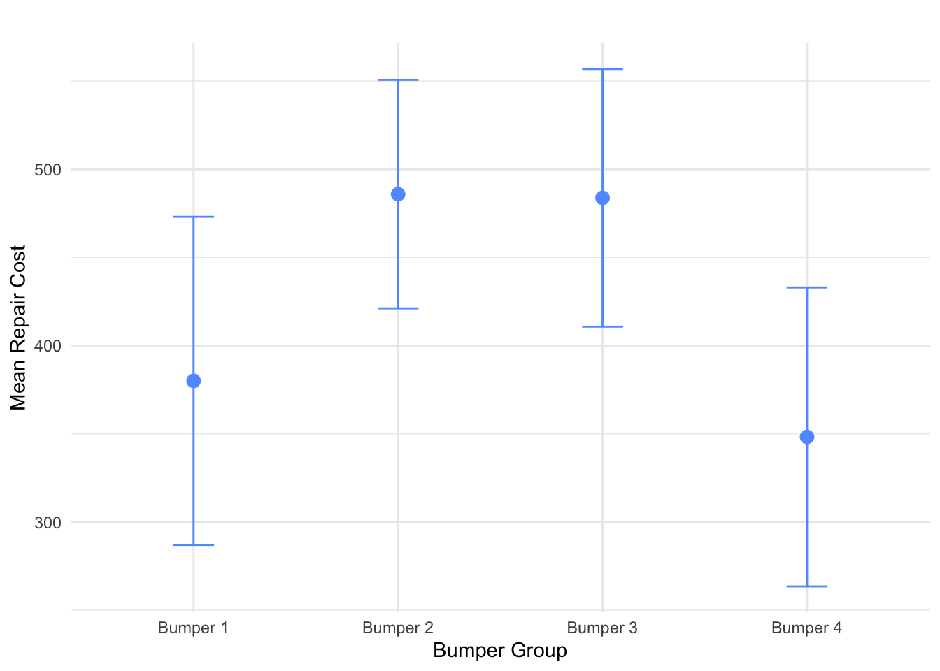
Figure 8.2: 95% Confidence Intervals for Mean Cost by Bumper Group
We want to calculate a 95% pairwise confidence interval for the difference between Bumper 1 and Bumper 2 using Fisher’s LSD and Bonferroni.
We test: \(\mu_1 - \mu_2\)
Fisher’s LSD Formula:
\[ (\bar{X}_1 - \bar{X}_2) \pm t_{(n - k,\ \alpha/2)} \cdot \sqrt{ MSE \left( \frac{1}{n_1} + \frac{1}{n_2} \right) } \]
Plug in:
\[ (380 - 485.9) \pm t_{(36,\ 0.025)} \cdot \sqrt{12399 \left( \frac{1}{10} + \frac{1}{10} \right)} \]
From R:
\[ = -105.9 \pm 2.028 \cdot \sqrt{12399 \cdot \left( \frac{1}{10} + \frac{1}{10} \right)} \]
\[ = -105.9 \pm 100.9942 \]
\[ = (-206.894,\ -4.9058) \]
Since the entire interval is negative, that is:
\[
\mu_1 - \mu_2 \leq 0
\]
Conclusion: Fisher’s LSD suggests \(\mu_2 > \mu_1\)
Bonferroni Formula:
\[ (\bar{X}_i - \bar{X}_j) \pm t_{(n - k,\ \alpha/(2m))} \cdot \sqrt{ MSE \left( \frac{1}{n_1} + \frac{1}{n_2} \right) } \]
Plug in:
\[ (380 - 485.9) \pm t_{(36,\ \alpha/2m)} \cdot \sqrt{12399 \left( \frac{1}{10} + \frac{1}{10} \right)} \]
Where:
\[ \alpha/2m = \frac{0.05}{2 \times 6} = 0.004167 \]
From R:
\[ = -105.9 \pm 2.79197 \cdot \sqrt{12399 \left( \frac{1}{10} + \frac{1}{10} \right)} = -105.9 \pm 139.0338 \]
\[ = (-244.9335,\ 33.13347) \]
Since the interval contains zero, that is:
\[ \mu_1 - \mu_2 \in (-244,\ 33) \]
Conclusion: Bonferroni informs us it is plausible that \(\mu_1 = \mu_2\)
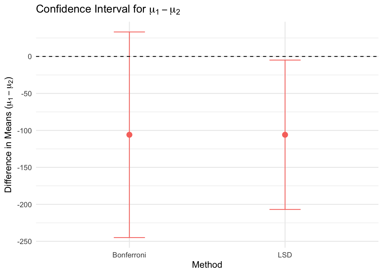
Figure 8.3: Comparison of LSD and Bonferroni Confidence Intervals for \(\mu_1 - \mu_2\). LSD is narrower; Bonferroni adjusts for multiple comparisons.
Using DescTools::PostHocTest() for Fisher’s LSD
We perform Fisher’s LSD post-hoc test using the DescTools package:
This returns the following multiple comparisons of means:
95% Family-wise Confidence Level – Fisher LSD
| Comparison | diff | lwr.ci | upr.ci | p-value |
|---|---|---|---|---|
| Bumper 2 - Bumper 1 | 105.9 | 4.9053 | 206.8947 | 0.0404 |
| Bumper 3 - Bumper 1 | 103.8 | 2.8053 | 204.7947 | 0.0443 |
| Bumper 4 - Bumper 1 | -31.8 | -132.7947 | 69.1946 | 0.5271 |
| Bumper 3 - Bumper 2 | -2.1 | -103.0947 | 98.8946 | 0.9666 |
| Bumper 4 - Bumper 2 | -137.7 | -238.6947 | -36.7054 | 0.0089 |
| Bumper 4 - Bumper 3 | -135.6 | -236.5947 | -34.6053 | 0.0099 |
Signif. codes: 0 ‘’ 0.001 ‘’ 0.01 ‘’ 0.05 ‘.’ 0.1 ‘ ’ 1
Using DescTools::PostHocTest() for Bonferroni Correction
We perform a Bonferroni-adjusted post-hoc test using the DescTools package:
This returns the following multiple comparisons of means:
95% Family-wise Confidence Level – Bonferroni
| Comparison | diff | lwr.ci | upr.ci | p-value |
|---|---|---|---|---|
| Bumper 2 - Bumper 1 | 105.9 | -33.1341 | 244.9341 | 0.2423 |
| Bumper 3 - Bumper 1 | 103.8 | -35.2341 | 242.8341 | 0.2657 |
| Bumper 4 - Bumper 1 | -31.8 | -170.8341 | 107.2341 | 1.0000 |
| Bumper 3 - Bumper 2 | -2.1 | -141.1341 | 136.9341 | 1.0000 |
| Bumper 4 - Bumper 2 | -137.7 | -276.7341 | 1.3341 | 0.0535 |
| Bumper 4 - Bumper 3 | -135.6 | -274.6341 | 3.4341 | 0.0595 |
Signif. codes: 0 ‘’ 0.001 ‘’ 0.01 ‘’ 0.05 ‘.’ 0.1 ‘ ’ 1
Bonferroni vs. LSD Comparison
| Bonferroni | LSD |
|---|---|
| Controls for experiment-wise error | Does not control for experiment-wise error |
| \(\alpha_E = 1 - (1 - \frac{\alpha}{m})^m\) | \(\alpha_E = 1 - (1 - \alpha)^m\) |
| Suitable when control of Type I error is required | Suitable when control of Type I error is not a strict concern |
| Higher risk of Type II error | Lower risk of Type II error |
| Lower power | Higher power |
Example
An apple juice manufacturer has developed a new product - a liquid concentrate that, when mixed with water, produces 1 liter of apple juice. The product has several attractive features. First, it is more convenient that canned apple juice. Second, because the apple juice that is sold in cans is actually made from concentrate, the quality of the new product is at least as high as canned apple juice. Third, the cost of the new product is slightly lower than canned apple juice. The marketing manager has to decide how to market the new product. She can create advertising that emphasizes convenience, quality, or price.
To facilitate a decision, she conducts an experiment. In three different cities that are similar in size and demographic makeup, she launches the product with advertising stressing the convenience of the liquid concentrate in one city. In the second city, the advertisements emphasize the quality of the product. Advertising that highlights the relatively low cost of the liquid concentrate is used in the third city. The number of packages sold weekly is recorded for the 20 weeks following the beginning of the campaign.
These data are available at:
The marketing manager wants to know if differences in sales exist between the three advertising strategies.
To illustrate Fisher’s LSD method and the Bonferroni adjustment, consider the dataset described above and assume we tested to determine whether population means differ using a \(5 \%\) significance level. The three sample means are: \(577.55,653.0\), and 608.65 . The pair-wise absolute differences are
\[ \begin{aligned} & \left|\bar{x}_{1}-\bar{x}_{2}\right|=|577.55-653.0|=|-75.45|=75.45 \\ & \left|\bar{x}_{1}-\bar{x}_{3}\right|=|577.55-608.65|=|-31.10|=31.10 \\ & \left|\bar{x}_{2}-\bar{x}_{3}\right|=|653.0-608.65|=|44.35|=44.35 \end{aligned} \]
If we conduct the LSD procedure with \(\alpha=0.05\) we find \(\left|t_{\alpha / 2, n-k}\right|=\left|t_{0.025,57}\right|=|-2.0024655|=2.0024655\)
\[
\text{LSD} = t_{\alpha / 2} \cdot \sqrt{MSE \left( \frac{1}{n_i} + \frac{1}{n_j} \right)}
\approx 2.002 \cdot \sqrt{8894 \left( \frac{1}{20} + \frac{1}{20} \right)} = 59.71
\]
We can see that only one pair of sample means differ by more than 59.71.
That is, \(|\bar{x}_1 - \bar{x}_2| = 75.45\), and the other two differences are less than LSD.
We conclude that only \(\mu_1\) and \(\mu_2\) differ.
If we perform the LSD procedure with the Bonferroni adjustment,
the number of pairwise comparisons is 3 (calculated as \(C = \frac{k(k - 1)}{2} = \frac{3(2)}{2}\)).
We set \(\alpha = 0.05 / 3 = 0.0167\). Thus,
\[
t_{\alpha/2,\, n-k} = t_{0.0083,\, 57} = -2.4682794
\]
and
\[ t_{\alpha / 2} \sqrt{M S E\left(\frac{1}{n_{i}}+\frac{1}{n_{j}}\right)} \approx 2.467 \sqrt{8894\left(\frac{1}{20}+\frac{1}{20}\right)}=73.54 \]
Again we conclude that only \(\mu_{1}\) and \(\mu_{2}\) differ. Notice, however, in the second calculation LSD is larger. The drawback to LSD is that we increase the probability of at least one Type I error. The Bonferroni adjustment corrects this problem.