Chapter 5 Next Generation Matrix
5.1 Introduction to the Chapter
This chapter describes in depth the use of the Next Generation Matrix (NGM) method. This tool is used to calculate the \(R_0\) value (Definition 1.3). Using the NGM achieves this this for multi-compartmental models (e.g. SEIR), by linearizing the system of differential equations around the Disease-Free Equilibrium (DFE) and dividing the flow of disease (Definition 3.1) into what causes new cases and what accounts for everything else that happens to an infected person. It is also important to mention that these tools are not limited to specific models and can be used for a variety of models. This chapter will use the SEIR model as an example for applying the NGM method (recall the SEIR model from Chapter 2.2.1).
5.2 Solving the SEIR Model
5.2.1 Definining the SEIR Model and Parameters
The SEIR model expands on our previous SIR model with the additional compartment “Exposed”. This compartment represents individuals in the population that have been infected, but are not yet infectious.

Figure 5.1: The SEIR compartmental model.
We begin by defining \(X\) as the vector of disease compartments. Then we can have: \[\frac{dX}{dt} = F(x) - V(x)\]
\(F(x)\) is a vector of the terms that lead to new infections
\(V(x) = V^- (x) -V^+ (x)\) where \(V^- (x)\) and \(-V^+ (x)\) contain all other outputs and inputs, respectively, for each disease compartment
For instance, the SIR model has \(X = \begin{bmatrix} I \end{bmatrix}\). We define \(X\) for the SEIR model as: \(X = \begin{bmatrix} E\\ I\\ \end{bmatrix}\).
We also define the differential equations for the SEIR model: \[ \begin{align*} \ \dot{S} &= - \beta SI \\ \ \dot{E} &= \beta SI - \delta E \\ \ \dot{I} &= \delta E - \gamma I \\ \ \dot{R} &= \gamma I \\ \end{align*} \]
5.2.2 Defining the Disease Free Equilibrium (DFE)
The Disease Free Equilibrium (Definition 3.3) exists when all infected compartments are set to 0. In other words, \(E=0\) and \(I=0\).
First, set all differential equations equal to zero. \[ \begin{align*} \ \dot{S} &= - \beta SI = 0\\ \ \dot{E} &= \beta SI - \delta E = 0 \\ \ \dot{I} &= \delta E - \gamma I = 0\\ \ \dot{R} &= \gamma I = 0\\ \end{align*} \] At the DFE:
- \(\dot{S} = 0\) is true when \(I=0\)
- \(\dot{E} = 0\) is true when \(I=0\) and \(E=0\)
- \(\dot{I} = 0\) is true when \(E=0\) and \(I=0\)
- \(\dot{R} = 0\) is true when \(I=0\)
Since there are no infections, \(E=I=R=0\). This means that for \(N=S+E+I+R\), \(N=S\) due to our earlier statements. So at the DFE for the \((S,E,I,R) = (N,0,0,0)\).
This is important for understanding later substitutions in the Chapter.
5.2.3 Solving SEIR Model with NGM
Recall that for the SEIR model the disease compartments are \(E\) and \(I\), so \(\dot{X} = \begin{bmatrix} \dot{E}\\ \dot{I}\\ \end{bmatrix}\).
Substitute the differential equations for \(\dot{E}\) and \(\dot{I}\) into \(X\).
\[ \begin{align*} \ \dot{X} &= \begin{bmatrix} \dot{E}\\ \dot{I}\\ \end{bmatrix} \\ \ \dot{X} &= \begin{bmatrix} \beta SI - \delta E \\ \delta E - \gamma I \\ \end{bmatrix} \\ \ \dot{X} &= \begin{bmatrix} \beta SI \\ 0 \\ \end{bmatrix} - \left( \begin{bmatrix} \delta E \\ \gamma I \\ \end{bmatrix} - \begin{bmatrix} 0 \\ \delta E \\ \end{bmatrix} \right) \\ \ \dot{X} &= F(x) - ( V^- (x) -V^+ (x) ) \\ \end{align*} \]
Note that the 0 in \(F(x) = \begin{bmatrix} \beta SI \\ 0 \\ \end{bmatrix}\) exists because \(F\) only considers brand new infected (the flow from \(S \rightarrow E\) and not \(S \rightarrow I\)). In other words, new infected are not necessarily infectious.
We separated \(\dot{X}\) into components to assist us in our \(R_0\) calculations.
For further simplicity, we also let: \(F(x) = \begin{bmatrix} \beta SI \\ 0 \\ \end{bmatrix} = \begin{bmatrix} F_1 \\ F_2 \\ \end{bmatrix}\), \(V(x) = \begin{bmatrix} \delta E \\ \gamma I - \delta E \\ \end{bmatrix} = \begin{bmatrix} V_1 \\ V_2 \\ \end{bmatrix}\)
Next, we find the Jacobian Matrices of \(F(x)\) and \(V(x)\) at the DFE. (Recall Jacobians from Chapter 4.2).
Let the Jacobian of F(x) be F.
\[ \boldsymbol{F} = J_F (x) = \begin{bmatrix} \frac{\partial F_1}{\partial E} & \frac{\partial F_1}{\partial I} \\ \frac{\partial F_2}{\partial E} & \frac{\partial F_2}{\partial I} \\ \end{bmatrix} = \begin{bmatrix} 0 & \beta S \\ 0 & 0 \\ \end{bmatrix} \]
Since we defined the DFE earlier as \((S,E,I,R) = (N,0,0,0)\), and we let population \(N = 1\), we then get \(S=1\) at DFE. Substituting \(S=1\) in, we get:
\[ J_F (x) = \begin{bmatrix} 0 & \beta \\ 0 & 0 \\ \end{bmatrix} \]
Let the Jacobian of V(x) be V.
\[ \boldsymbol{V} = J_V (x) = \begin{bmatrix} \frac{\partial V_1}{\partial E} & \frac{\partial V_1}{\partial I} \\ \frac{\partial V_2}{\partial E} & \frac{\partial V_2}{\partial I} \\ \end{bmatrix} = \begin{bmatrix} \delta & 0 \\ -\delta & \gamma \\ \end{bmatrix} \]
Another way to think about it: \(\dot{X} = (f-v) \begin{bmatrix} E \\ I \end{bmatrix} = (f-v)X\)
We will now find the NGM.
Definition 5.1 (Next Generation Matrix (NGM) method) A method to determine the \(R_0\) value for compartmental models.
Formula: \(NGM = \boldsymbol{F} \boldsymbol{V}^{-1}\)
Using the NGM formula from (Definition 5.1), we obtain the NGM for the SEIR model with our previously determined F and V.
To find \(\boldsymbol{V} ^{-1}\) we use the following rule:
for matrix \(M = \begin{bmatrix} a & b \\ c & d \\ \end{bmatrix}\), the inverse matrix is \(M^{-1} = \frac{1}{ad-bc} \begin{bmatrix} d & -b \\ -c & a \\ \end{bmatrix}\)
Then, we have \(\boldsymbol{F} = \begin{bmatrix} 0 & \beta \\ 0 & 0 \\ \end{bmatrix}\) and \(\boldsymbol{V} ^{-1} = \frac{1}{\delta \gamma} \begin{bmatrix} \gamma & 0 \\ \delta & \delta \\ \end{bmatrix}\)
\[ \begin{align*} \ NGM = \boldsymbol{F} \boldsymbol{V} ^{-1} &= \begin{bmatrix} 0 & \beta \\ 0 & 0 \\ \end{bmatrix} \frac{1}{\delta \gamma} \begin{bmatrix} \gamma & 0 \\ \delta & \delta \\ \end{bmatrix} \\ \ &= \begin{bmatrix} 0 & \beta \\ 0 & 0 \\ \end{bmatrix} \begin{bmatrix} \frac{1}{\delta} & 0 \\ \frac{1}{\gamma} & \frac{1}{\gamma} \\ \end{bmatrix} \\ \ &= \begin{bmatrix} \frac{\beta}{\gamma} & \frac{\beta}{\gamma} \\ 0 & 0 \\ \end{bmatrix} \\ \end{align*} \]
Refer back to the formula in Chapter 4.2.1.1, where \(det(J-\lambda I_n) = 0\). \(R_0\) is the spectral radius (i.e. largest eigenvalue) of \(\ \boldsymbol{F} \boldsymbol{V} ^{-1}\).
\[ det \left( \begin{bmatrix} \frac{\beta}{\gamma} - \lambda & \frac{\beta}{\gamma} \\ 0 & - \lambda \\ \end{bmatrix} \right) = - \lambda \left( \frac{\beta}{\gamma} - \lambda \right) \]
Let \(- \lambda \left( \frac{\beta}{\gamma} - \lambda \right) = 0\).
So \(\lambda = 0\) and \(\lambda = \frac{\beta}{\gamma}\). The latter is the largest eigenvalue, so \(R_0 = \lambda = \frac{\beta}{\gamma}\). Thus, we have obtained the \(R_0\) using the NGM method.
5.3 Solving the SEIR Model with Birth and Death
In this version of the SEIR model, demographic effects such as births and deaths (also known as vital dynamics) are included to increase model realism.
\(\mu N\) represents births
\(\mu\) represents deaths
The birth term \(\mu N\) adds to the susceptible population, while the deaths occur at a rate \(\mu\) across the four compartments.
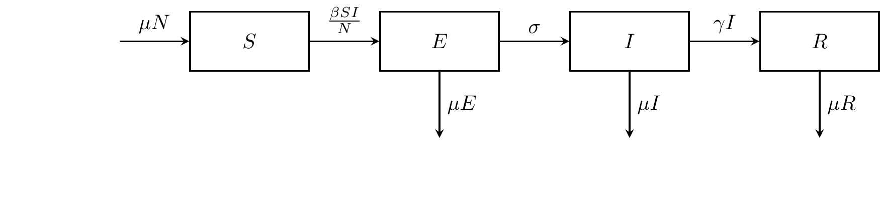
Figure 5.2: The SEIR compartmental model.
The four differential equations for the SEIR model with vital dynamics can then be constructed. Also recall that \(S+E+I+R=N\).
\[ \begin{align*} \dot{S} &= \mu N - \frac{\beta SI}{N} \\ \dot{E} &= \frac{\beta SI}{N} - (\sigma + \mu)E \\ \dot{I} &= \sigma E - (\gamma + \mu)I \\ \dot{R} &= \gamma I - \mu R \\ \end{align*} \]
At the Disease-Free Equilibrium (DFE), there are no infections (\(E = 0\) and \(I = 0\)). We then set all differential equations equal to 0, and \(E = 0\) and \(I = 0\). Therefore at the DFE, we obtain \(\dot{S} = 0\) when \(S = N\), which means the entire population is susceptible. We use this equilibrium to linearize the system and separate infection terms (\(F(x)\)) from other transition terms (\(V(x)\)).
\[ \begin{align*} \dot{X} &= F(x) - V(x) \\ &= \begin{bmatrix} \frac{\beta SI}{N} \\ 0 \end{bmatrix} - \begin{bmatrix} (\sigma + \mu)E \\ (\gamma + \mu)I - \sigma E \end{bmatrix} \end{align*} \]
Here, the first vector \(F(x)\) captures new infections — in this case, the flow from the susceptible compartment \(S\) to the exposed compartment \(E\). The second vector, \(V(x)\), represents all other movements between infected compartments (progression, recovery, and death).
The Jacobian of \(F(x)\) is the following, where the right-most matrix is obtained when \(S = N\) at DFE: \[ \boldsymbol{F} = J_F (x) = \begin{bmatrix} 0 & \frac{\beta S}{N} \\ 0 & 0 \end{bmatrix} = \begin{bmatrix} 0 &\beta \\0&0 \end{bmatrix} \] The Jacobian of \(V(x)\) is \[ \boldsymbol{V} = J_V (x) = \begin{bmatrix} \sigma + \mu & 0 \\ -\sigma & \gamma + \mu \end{bmatrix} \]
Lastly, we obtain the NGM by following Definition 5.1:
\[
\begin{align*}
NGM = \boldsymbol{F}\boldsymbol{V}^{-1} &=
\begin{bmatrix}
0 & \beta \\
0 & 0
\end{bmatrix}
\frac{1}{(\sigma + \mu)(\gamma + \mu)}
\begin{bmatrix}
\gamma + \mu & 0 \\
\sigma & \sigma + \mu
\end{bmatrix} \\
&=
\begin{bmatrix}
\frac{\beta \sigma}{(\sigma + \mu)(\gamma + \mu)} & \frac{\beta}{\gamma + \mu} \\
0 & 0
\end{bmatrix}
\end{align*}
\]
Multiplying \(F\) by \(V^{-1}\) captures how many new infections one infected individual generates in each compartment over their infectious period.
The resulting matrix describes the expected number of new infections caused by an exposed or infectious person.
The basic reproduction number \(R_0\) is given by the the largest eigenvalue of the next generation matrix. Therefore: \(R_0 = \frac{\beta \sigma}{(\sigma + \mu)(\gamma +\mu)}\)
This value shows how the disease’s ability to spread depends not only on transmission (\(\beta\)) and recovery (\(\gamma\)), but also on the rates of progression (\(\sigma\)) and death (\(\mu\)). If \(\mu = 0\), meaning no births or deaths occur, this expression simplifies to \(R_0 = \frac{\beta}{\gamma}\) which is the classic SIR result.
References: [2]
5.4 Visualizing the SEIR Models
Below, we have time series plots displaying the two examples we have looked at in this chapter. We used the following parameters in these plots:
initial population size: \(N = 500\)
transmission rate: \(\beta = 0.4\)
progression rate from exposed to infected: \(\delta = \sigma = 0.27\)
recovery rate: \(\gamma = 0.10\)
death rate: \(\mu = 0.0001\) (only used in Figure 5.4)
Figures 5.3 and 5.4 visualize the differences on a disease model that the presence of vital dynamics can have, despite the rest of the parameters being the same. Also, note the difference in the time scales between the plots. The plot without vital dynamics (Figure 5.3) is simulated over a period of 75 days, while the plot including vital dynamics (Figure 5.4) is simulated over a period of 1 year.
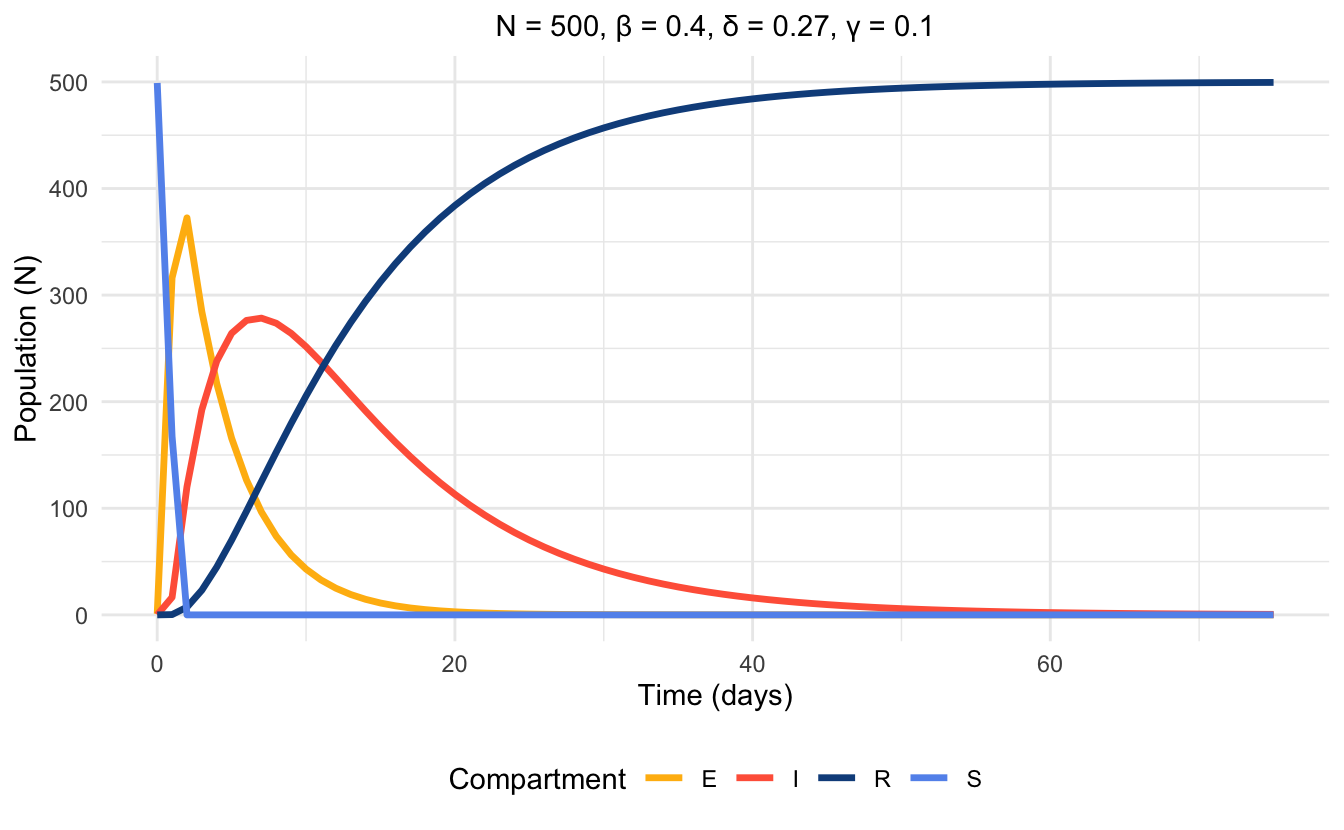
Figure 5.3: Time series plot of SEIR model without vital dynamics at endemic equilibrium, simulated with parameter values.
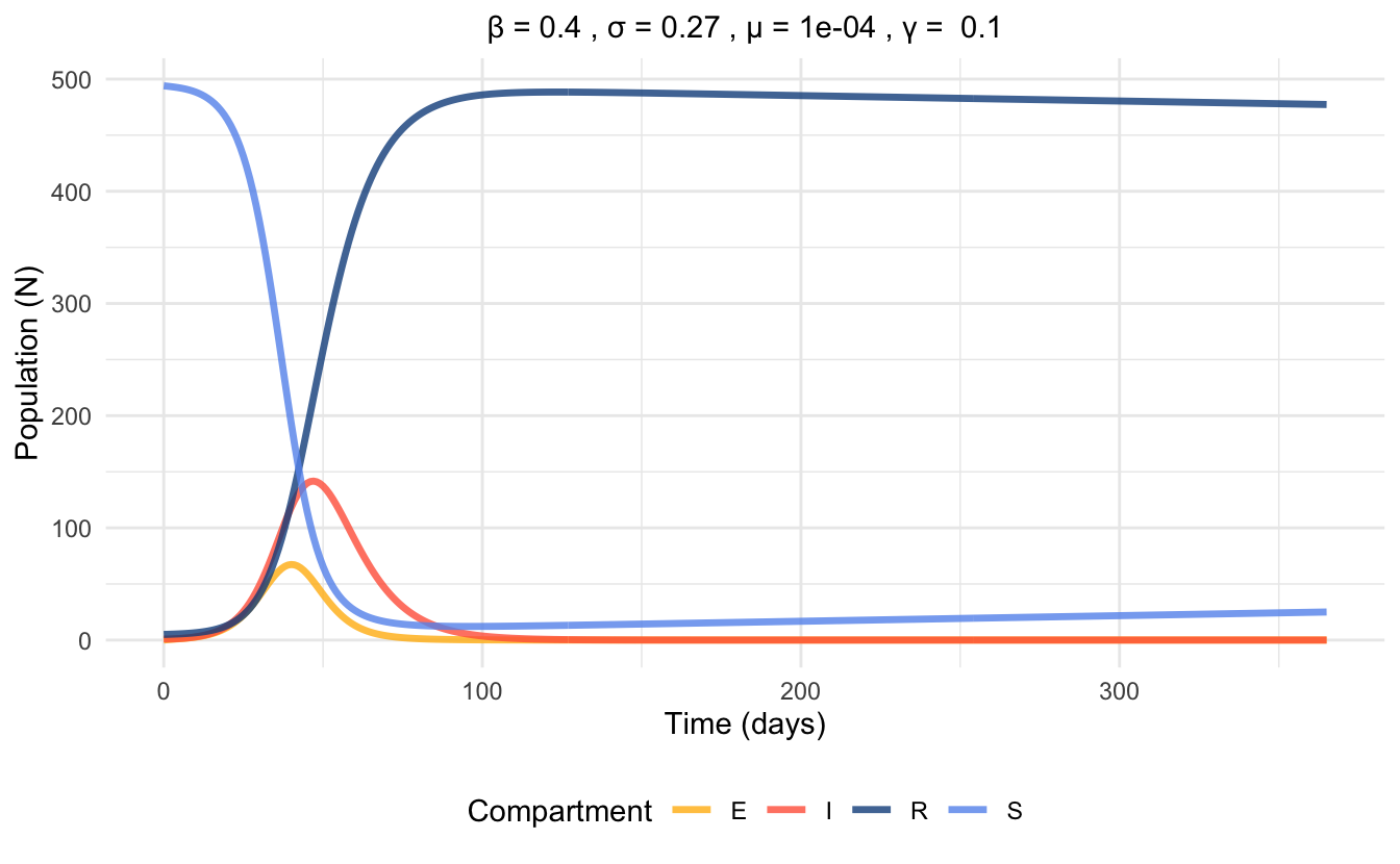
Figure 5.4: Time series plot of SEIR model with vital dynamics at endemic equilibrium, simulated with parameter values.