Chapter 3 Modelling Disease Dynamics with ODEs
3.1 Introduction to the Chapter
Chapter 3 examines various aspects of the basic compartmental models: the SI model and the SIR model. In this chapter we will define model parameters and the flow between compartments. We will also seek mathematical solutions to the models to gain a comprehensive understanding of model initialization, functionality, and interpretation. The concepts discussed in this chapter provide a foundation for further analysis of epidemiological models explored in later chapters of this book.
3.2 Interactions Between Compartments
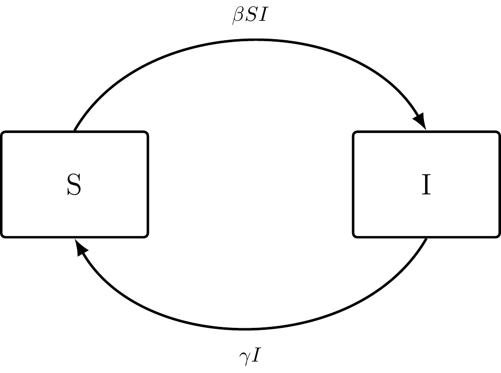
Figure 3.1: The SI compartmental model.
Defining Parameters:
S : Proportion of population that is susceptible (Definition 2.5).
I : Proportion of population that is infected (Definition 2.6).
N : Total Population
Differentials (\(\frac {dS}{dt}\) and \(\frac {dI}{dt}\)): Net Flow of individuals in and out of specific compartments
\(\beta SI\): Total Rate of New Infections in a Population
- \(\beta\): Transmission Rate
\(\gamma I\): Recovery Rate of Infectious Individuals
- \(\gamma\): Recovery Rate
Now that each term of the equation is defined, we can start to understand the interactions occurring. First we will dive into the meaning of the signage of each term:
Positive (+): Represents Inflow; Adding individuals to a compartment
Negative (-): Represents Outlfow; Removing individuals from a compartment
Definition 3.1 (Flow) Flow is the movement of people move from one compartment to another.
Compartmental models (Definition 2.3) are designed specifically to illustrate flow. Below are equations representing the net flow of individuals into and out of Susceptible (Definition 2.5) and Infectious (Definition 2.6) compartments, respectively. This flow is represented by the differential in both equations.
\[ \frac {dS}{dt} = -\beta SI + \gamma I \]
\[ \frac {dI}{dt} = +\beta SI - \gamma I \]
The signs in each equation indicate the direction of flow between compartments. For instance, \(-\beta SI\) represents the loss of susceptible individuals as they become infected, while \(+\beta SI\) represents the corresponding gain in the infectious group. The same relationship applies to \(\gamma I\), which describes the recovery process in reverse.
Understanding the parameters and signage then, one can understand the equations above. \(\frac {dS}{dt}\) calculates the net flow of the susceptible group by subtracting the total rate of new infections in a population (the proportion of the population entering the infected compartment) and by adding the recovery rate of infectious individuals (the proportion of the population entering the susceptible compartment). \(\frac {dI}{dt}\) calculates the net flow of the infected group by adding the total rate of new infections in a population (the proportion of the population entering the infected compartment) and by subtracting the recovery rate of infectious individuals (the proportion of people entering the susceptible compartment). These simple SI equations form the foundation for more complex models, such as SIR or SEIR, which introduce additional compartments to capture recovery, immunity, or incubation dynamics. [21]
3.3 Solving the SI Model
In the SIS model, it is assumed that an individual is either susceptible (Definition 2.5) or infected (Definition 2.6) and this means once an individual has recovered from the infection they return to the susceptible group. In this work through, it is assumed that the population stays roughly constant.
The goal of solving the SIS model is to understand and predict the spread of an infectious disease within a population. Analyzing differential equations can help predict disease prevalence over time and determine whether a disease is endemic (Definition 1.2) or not. In addition, the differential equations can also be used to identify the size of infected (Definition 2.6) and susceptible (Definition 2.5) populations at the stable endemic state. By solving the differential equations, \(S(t)\) and \(I(t)\) can be found and used to predict the size of the susceptible and infected compartments at different periods in time.
These are the initial assumptions in equation format, showing that within the population, an individual can either be in the susceptible or infected compartment. Together both compartments make up the total population, \(N\). \[ S+I=N \]
In many of the compartmental models in this textbook, we let the populations be represented as a proportion, so \(N = 1\). As a result, \(S\) and \(I\) are both proportions of the population.
\[ S+I=1 \] Rearranging this equation finds: \[ I=1-S \]
Deriving both of the previous equations creates a system of differential equations:
\[ \frac {dS}{dt} = -\beta SI + \gamma I \]
\[ \frac {dI}{dt} = \beta SI - \gamma I \]
Reduce the system of 2 equations to just 1 by plugging in \((1-S)\) for \(I\): \[ \frac {dS} {dt}= -\beta S(1-S) + \gamma (1-S) = (\gamma - \beta S)(1-S) \]
After separating the variables, we can take an integral of both sides to determine \(S(t)\).
\[ \int \frac {1}{(\gamma - \beta S)(1-S)} dS = \int dt \]
Partial Fractions can be used to solve this integral:
\[ \frac {A}{\gamma - \beta S} + \frac {B}{1-S}= \frac {A(1-S)+B( \gamma - \beta S)}{( \gamma - \beta S)(1-S)} \]
So then: \[ A(1-S)+B( \gamma - \beta S) = 1 \]
In order to solve this equation, one can assume:
\[ A + \beta \gamma = 1 \]
\[ A + B \beta =0 \]
Through partial fractions it will be found that: \[ A = \frac {1}{\beta - \gamma } \]
\[ B = \frac {1}{\gamma - \beta} \]
Plugging in the new \(A\) and \(B\): \[ \int \frac{1}{(\gamma - \beta S)(1-S)} dS = \int \frac{\beta}{\beta - \gamma}\left(\frac {1}{\gamma - \beta S}\right) + \frac{1}{\gamma - \beta}\left(\frac {1}{1-S}\right)dS \]
Solving the integral on the left side first results in:
\[ \int \frac{1}{(\gamma - \beta S)(1-S)} dS = \int \frac{\beta}{\beta - \gamma}\left(\frac {1}{\gamma - \beta S}\right) + \frac{1}{\gamma - \beta}\left(\frac {1}{1-S}\right)dS = \frac {1}{\gamma - \beta} \ln \left| \frac{\gamma - \beta S}{1-S} \right| \]
Solving the integral on the right side results in:
\[ \int dt = t +C \] Therefore the new equation is: \[ \frac {1}{\gamma - \beta} \ln \left| \frac{\gamma - \beta S}{1-S} \right| = t+C \]
Solving for \(S(t)\) finds:
\[ S(t)= \frac {\gamma - Ce^{(\gamma - \beta )t}}{\beta - Ce^{(\gamma - \beta)t}} \]
Then plugging in \(t=0\) and using \(S_0\) to solve for the constant :
\[ S(0) = \frac {\gamma - C}{\beta -C} \]
\[ S_0(\beta - C) = \gamma -C \]
\[ S_0 \beta - \gamma = C(S_0 -1) \]
\[ C = \frac{S_0 \beta - \gamma}{S_0 -1} \] Plugging \(C\) into \(S(t)\) results in the final equation for \(S(t)\): \[ S(t)= \frac {\gamma - (\frac{S_0 \beta - \gamma}{S_0 -1}) e^{(\gamma - \beta )t}}{\beta - (\frac{S_0 \beta - \gamma}{S_0 -1})e^{(\gamma - \beta)t}} \]
Thus through this work through of the SIS model, we have found a closed form solution for \(S(t)\), which shows the number or proportion of individuals in the susceptible compartment at a time t. Using the function found for \(S(t)\), one can plug it into the assumption equations, specifically \(I+S=1\), in order to find \(I(t)\). In addition, learning from this model, one can note that when \(\beta > \gamma\), transmission is greater than recovery so there will be a spread of the infections and the disease will be endemic. However, when \(\beta < \gamma\), recovery occurs faster than transmission and the disease will die out.
Solving the SIS model not only provides a solution for \(S(t)\) and \(I(t)\), but also will provide a groundwork for more complex models, such as the SIR model .
3.4 Solving the SIR Model
Building what we have learnt previously from solving the SI model, we will now attempt to solve the SIR model.
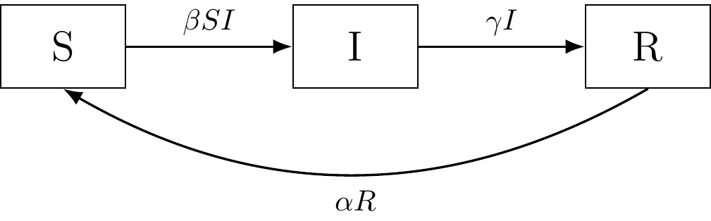
Figure 3.2: The SIR compartmental model.
The SIR model includes a new compartment, “R”, which represents recovery from infection; or alternatively, those removed from infection status. This removal can occur as a result of immunization from infection, immunity from recovering from the disease, isolation from the population, or death. Note that the latter demographic effects (birth/death) are not observed in our example, and different models can exist for those cases.
We define a new system of differential equations for the SIR model as follows:
\(\displaystyle\frac{dS}{dt} = - \beta SI + \alpha R\)
\(\displaystyle\frac{dI}{dt} = \beta SI - \gamma I\)
\(\displaystyle\frac{dR}{dt} = \gamma I - \alpha R\)
Defining the parameters: As before, the differentials represent the net flow of individuals in and out of compartments, and \(\beta\) represents infection rate (S to I). \(\gamma\) represents recovery rate of the infected, but now individuals moving out of compartment “I” (infected) move into compartment “R” (recovered/removed). \(\alpha\) is a new term in the equations that represents the re-susceptible rate where recovered individuals lose immunity and become susceptible again (R to S).
Note that \(S,I,R \in [0,1]\). If the population is represented by \(N = S + I + R\), we can let \(N = 1\) and get \(S + I + R = 1\). So \(R = 1 - S - I\).
Plugging into the system of equations we get:
\[ \frac{dS}{dt} = - \beta SI + 2(1 - S - I) \]
However, unlike the SI model, the SIR model’s system of equations has no closed form solution. Instead, we can find the equilibrium for this system. This system is considered to be a dynamical system, and our analysis will be qualitative.
Definition 3.2 (Equilibrium) The rate of individuals entering a compartment is equal to the rate of individuals leaving a compartment.
Thus, we can set each equation in our system of equations to 0.
The new system of equations at equilibria:
\(0 = -\beta SI + \alpha R\)
\(0 = \beta SI - \gamma I \Rightarrow 0 = (\beta S - \gamma) I\)
\(0 = -\gamma I + \alpha R\)
There are two types of equilibrium in epidemiology:
Definition 3.3 (Disease Free Equilibria (DFE)) There are no infected in the population, so \(I* = 0\) in our SIR model (notation: asterix indicates equilibrium solution)
Definition 3.4 (Endemic Equilibria (EE)) Infected (Definition 2.6) persist indefinitely, so \(I* > 0\) in our SIR model (notation: asterix indicates equilibrium solution)
First we solve for DFE. From equation 2 we get: \(I = 0\), or \(S=\frac{\gamma}{\beta}\)
Then plugging in \(I = 0\) into the system of equations:
\(0 = \alpha R\)
\(0 = -\alpha R\)
Solving for \(R\) from these 2 equations, we get \(R^* = 0\)
Since \(R = 1 - S - I\), \(R^* = 0\), and \(I = 0\), then \(S^* = 1\) (note: another way to write \(S^*\) is \(\overline S\)). We use the asterisk or bar to indicate equilibrium notation.
Therefore, at Equilibrium (Definition 3.2):
\[ (S^*, I^*) = (1, 0) \]
Thus, at DFE (Definition 3.3), the entire population is susceptible to infection and no EE (Definition 3.4) exists because the infectious population returns to zero once the endemic is over.
Now, we solve for EE. Plugging \(S = \frac{\gamma}{\beta}\) into the system of equations (equation 3):
\[ \begin{align*} \ 0 &= -\gamma I + \alpha \left(1 - \frac{\gamma}{\beta} - I \right) \\ \ 0 &= \gamma I - \alpha \left(1 - \frac{\gamma}{\beta} - I \right) \\ \ \alpha \left(1 - \frac{\gamma}{\beta} \right) &= I (\gamma + \alpha) \end{align*} \]
Solving for I we get:
\[ I^* = \frac{\alpha (1 - \frac{\gamma}{\beta})}{\gamma + \alpha} \]
Endemic equilibrium (EE) (Definition 3.4) is:
\[ (S^*, I^*) = \left( \frac{\gamma}{\beta}, \frac{\alpha (1- \gamma/\beta)}{\gamma + \alpha} \right) \]
where \(\gamma < \beta\).
EE (Definition 3.4) requires a continuous supply of susceptible (Definition 2.5) (“susceptible replacement”), for instance, by birth, or reduced immunity to the disease. Otherwise, I will approach 0 after the endemic.
Also, since \(\gamma < \beta\), we get \(R_0 = \frac{\beta}{\gamma} > 1\). The basic reproduction number (\(R_0\)) (Definition 1.3) is a threshold quantity that indicates the occurrence of an epidemic. \(R_0\) can also be thought of as the number of secondary infections caused by a single infected (Definition 2.6) individual in a population of susceptible (Definition 2.5) individuals (e.g. at initial time \(t = 0\)). Note that individual variation is excluded in the definition.
Specific values of \(R_0\) (Definition 1.3) can be used to analyze the stability of equilibrium (Definition 3.2). This will be discussed in further detail in Chapter 4, but more generally for now:
If \(R_0 < 1\): DFE is stable, the infection dies out (i.e. when infected, an individual infects less than one person on average, then the disease dies out)
If \(R_0 > 1\): EE is stable, there is an epidemic (i.e. when infected, an individual infects more than one person on average, then the disease spreads)
3.4.1 Effective Reproduction Number
While the basic reproduction number (\(R_0\)) represents the average number of secondary infections generated by a single infected individual in a completely susceptible population, this assumption rarely holds true in real-world outbreaks. Over time, as immunity builds and interventions are introduced, the actual transmission potential changes. To capture this dynamic, epidemiologists use the effective reproduction number, \(R_e\) (or \(R_t\) measured at a time t).
Definition 3.5 (Effective Reproduction Number) \(R_e\) quantifies the number of secondary cases expected per infection at time \(t\), accounting for the current level of susceptibility and external factors such as vaccination, behavioral changes, or public health measures.
Going forward this will be our more detailed definition of \(R_e\). It is related to \(R_0\) through the proportion of the population that remains susceptible:
\[ R(t) = \frac{S(t)}{S(0)} R_0 \] This equation shows the temporal decline in the epidemic (Definition 1.1) due to depletion of susceptible (Definition 2.5) individuals.
Monitoring \(R_e\) (Definition 3.5) over time provides a statistical framework for assessing how disease transmission responds to interventions or natural immunity accumulation. In this sense, \(R_e\) serves as a bridge between theoretical epidemic models and real-time epidemiological data, allowing researchers to evaluate and predict time-dependent trends in disease spread. [17]
3.4.2 Interactive Dashboard
The dashboard below is a time series plot for the SIR model, where the populations present in each compartment (S, I, or R) change over time as individuals move between the compartments. Adjust the initial conditions or parameters of the dashboard to see the different time series plots that could exist for the SIR model.