Chapter 6 Extended Compartmental Models: Real World Applications and Solutions
6.1 Introduction to the Chapter
In this chapter, we will solve a variety of four-compartment models of varying complexity: the SIQR, SVIR, and SAIR models. These models are derived from scholarly articles and experiments in which the parameters, variables, and differential equations are provided. In this, we can apply our knowledge and techniques from previous chapters to analyze different compartmental models. After solving and analyzing these models, we will also look at some specific examples to understand the usage of these models with real data.
6.2 The SIQR Model
This model is based on the parameters and variables defined in the article by Kalachev et al. (2023) and is used to model COVID-19. [12]
The “Q” compartment represents quarantined individuals.
It is important to note that the authors state their limitations, as they do not include an “E” (Exposed) compartment. This means that the complexities of the case in question, COVID-19, is not fully modeled. However, for our purposes, this pre-existing model provides definitive parameters and variables to be manipulated and solved.

Figure 6.1: The SIQR compartmental model.
6.2.1 Defining the Parameters
\(\alpha\): infection rate
\(\beta\): quarantine rate
\(\gamma\): recovery rate
Beginning with X, the vector of disease compartments. For the SIQR model, \(X = \begin{bmatrix} I\\ Q\\ \end{bmatrix}\)
Refer back to the definitions of the new infection vector \(F(x)\) and the transition vector \(V(x)\) in Chapter 5.2.1.
6.2.2 Defining the Disease Free Equilibrium
Due to the closed system definition of the article, this SIQR Compartmental Model can only be solved at the DFE. This is due to the nature of a closed system in which the disease has already dissipated, thus, the Endemic Equilibrium cannot exist. However, modifications to create an open system with birth and death rates incorporated, an Endemic Equilibrium can then be solved for.
The Disease Free Equilibrium exists when all infected compartments (I and Q), are set to 0. Thus, \(I=0\) and \(Q=0\). So: \[ \begin{align*} \dot{S} &= -\alpha S I = 0\\ \dot{I} &= \alpha S I - \beta I = 0 \\ \dot{Q} &= \beta I - \gamma Q = 0 \\ \dot{R} &= \gamma Q = 0 \\ \end{align*} \] At the DFE:
- \(\dot{S}\) is true when \(I=0\)
- \(\dot{I}\) is true when \(I=0\)
- \(\dot{Q}\) is true when \(I=0\) and \(Q=0\)
- \(\dot{R}\) is true when \(Q=0\)
Since there are no infections: \(I=Q=R=0\) This means that for \(N=S+I+Q+R\), \(N=S\) due to our earlier statements So at the DFE for the \((S,I,Q,R) = (S,0,0,0) = (N,0,0,0)\)
It is important to note that we normally use \(\beta\) for the transmission parameter, while in this example it is \(\alpha\). Additionally \(\beta\) becomes the quarantine rate and \(\gamma\) remains as the recovery rate.
6.2.3 Solving the SIQR Model
6.2.3.1 Defining F and V Matrices
Recall: that for the SIQR model the disease compartments are I and Q:
\(\dot{X} = \begin{bmatrix} \dot{I}\\ \dot{Q}\\ \end{bmatrix}\)
In order to define the distinction between new infections and transferred compartments, we create 2 matrices: Transmission (F) and Transition (V)
- Transmission Matrix (F)
- In this Matrix, only compartments in which new infections are created \[ \begin{align*} \ F(x) &= \begin{bmatrix} \dot{I}\\ \dot{Q}\\ \end{bmatrix} \\ \ F(x) &= \begin{bmatrix} \alpha S I - \beta I \\ \beta I - \gamma Q \\ \end{bmatrix} \\ \ F(x) &= \begin{bmatrix} \alpha S I \\ 0 \\ \end{bmatrix} \end{align*} \]
- Transition Matrix (V)
- In this Matrix, using \(V = V^- + V^+\), we can find the transfer of infected individuals in and out of infected compartments
- We can see this transfer as each of the values stated below leave/subtracted from a differential equation of a compartment and enter/added to the differential equation of the next compartment \[ \begin{align*} \ V(X) &= \begin{bmatrix} \beta I \\ -\beta I + \gamma Q \\ \end{bmatrix} \\ \end{align*} \]
Referring back to Chapter 5.2.1 once again for the equation for \(\dot{X} = F(x) - V(x)\), we combine these matrices into:
\[ \begin{align*} \ \dot{X} &= \begin{bmatrix} \alpha S I \\ 0 \\ \end{bmatrix} - \begin{bmatrix} \beta I \\ -\beta I + \gamma Q \\ \end{bmatrix} \end{align*} \] For simplicity in later calculations: \[ \begin{align*} \ F(x) &= \begin{bmatrix} \alpha S I \\ 0 \\ \end{bmatrix} = \begin{bmatrix} F_1 \\ F_2 \end{bmatrix} \\ \ V(x) &= \begin{bmatrix} \beta I \\ -\beta I + \gamma Q \\ \end{bmatrix} = \begin{bmatrix} V_1 \\ V_2 \end{bmatrix} \end{align*} \]
6.2.3.2 Taking the Jacobian Matrix of F and V
Let the Jacobian of F(x) be F.
\[ \boldsymbol{F} = J_F (x) = \begin{bmatrix} \frac{\partial F_1}{\partial E} & \frac{\partial F_1}{\partial I} \\ \frac{\partial F_2}{\partial E} & \frac{\partial F_2}{\partial I} \\ \end{bmatrix} = \begin{bmatrix} \alpha S & 0\\ 0 & 0 \\ \end{bmatrix} \] At DFE, \(S = 1\)
- This is found by our earlier definition of the DFE.
- At the DFE for \((S,I,Q,R) = (S,0,0,0) = (N,0,0,0)\)
- Since Population \("N"=1\) and \(S=N\), then \(S=1\)
- So after subsituting \(S=1\):
\[ J_F (x) = \begin{bmatrix} \alpha S & 0 \\ 0 & 0 \\ \end{bmatrix} \]
Let the Jacobian of V(x) be V. \[ \boldsymbol{V} = J_V (x) = \begin{bmatrix} \frac{\partial V_1}{\partial E} & \frac{\partial V_1}{\partial I} \\ \frac{\partial V_2}{\partial E} & \frac{\partial V_2}{\partial I} \\ \end{bmatrix} = \begin{bmatrix} \beta & 0 \\ -\beta & \gamma \\ \end{bmatrix} \]
6.2.3.3 Finding the Next Generation Matrix
Refer to Chapter 5.2.3 where the NGM for the SEIR model is found. We will be using a similar structure once again. \(NGM = \boldsymbol{F} \boldsymbol{V}^{-1}\)
Thus: \[ \boldsymbol{F} = \begin{bmatrix} \alpha S & 0 \\ 0 & 0 \\ \end{bmatrix} \] For \(\boldsymbol{V}^{-1}\), we use the same inverse matrix rule.
\[\begin{align*} \boldsymbol{V} &= \begin{bmatrix} \beta & 0 \\ -\beta & \gamma \\ \end{bmatrix}\\ \boldsymbol{V}^{-1} &= \frac{1}{ad-bc} \begin{bmatrix} d & -b \\ -c & a \\ \end{bmatrix} \\ \boldsymbol{V}^{-1} &=\frac{1}{\beta \gamma} \begin{bmatrix} \gamma & 0 \\ \beta & \beta \\ \end{bmatrix}\\ \boldsymbol{V}^{-1} &= \begin{bmatrix} \frac{1}{\beta} & 0 \\ \frac{1}{\gamma} & \frac{1}{\gamma} \\ \end{bmatrix}\\ \end{align*}\]
So \(\boldsymbol{F} \boldsymbol{V}^{-1}\) is: \[ \begin{align*} \boldsymbol{F} \boldsymbol{V}^{-1} &= \begin{bmatrix} \alpha S & 0 \\ 0 & 0 \\ \end{bmatrix} \begin{bmatrix} \frac{1}{\beta} & 0 \\ \frac{1}{\gamma} & \frac{1}{\gamma} \\ \end{bmatrix} \\ \boldsymbol{F} \boldsymbol{V}^{-1} &= \begin{bmatrix} \frac{\alpha S}{\beta} & 0 \\ 0 &0 \\ \end{bmatrix} \end{align*} \]
6.2.3.4 Calculating \(R_0\) and Defining Stability
As stated previously in (Chapter 5.2.3), \(R_0\) is the spectral radius of the Next Generation Matrix \(\ \boldsymbol{F} \boldsymbol{V}^{-1}\) \[ det \left( \begin{bmatrix} \frac{\alpha S}{\beta} - \lambda & 0 \\ 0 & - \lambda \\ \end{bmatrix} \right) = - \lambda \left( \frac{\alpha S}{\beta} - \lambda \right) \] Let \(- \lambda \left( \frac{\alpha S}{\beta} - \lambda \right) = 0\) (\(\lambda_1\) and \(\lambda_2\) respectively)
So \(\lambda_1 = 0\) and \(\lambda_2 = \frac{\alpha S}{\beta}\). \(\lambda_2\) is the largest eigenvalue, so \(R_0 = \frac{\alpha S}{\beta}\).
Thus:
If \(R_0 < 1\) then the DFE is stable, and the disease dies out
- This means that \(\alpha S < \beta\)
If \(R_0 > 1\) then the DFE is unstable, and an epidemic occurs
- This means that \(\alpha S > \beta\)
6.2.4 Example with Parameter Values and Simulation
Throughout this textbook, we have discussed how to solve and understand varying models on a theoretical level. However; we are also able to fit these models to data in with certain datasets. To do this, we will use a very commonly used example in the world of applied epidemiology, the 1978 Influenza Outbreak in a British Boarding School. The data contained total cases, quarantined defined as “Confined to Bed,” and Recovering defined as “Convalescent.” This was a closed system and contained detail reports to understand what occurred using our modern techniques and models. Doing so allows us to map the data into the variables of our models and understand the situation from which our data was recorded.[12]
Parameter Values
Our normal parameter values \(\beta, \gamma, \alpha\) are derived using a MATLAB Optimization Toolbox
By giving the solver the total population, N, which is 763 in this scenario, and setting the initial infected, I(0) equal to 1, the software can create predicted curves
By minimizing the Standard Squared Error between the predicted curves and data points, the values of the parameters can be found
Fitting the SIQR Model
When fitting this model, there were two clear ways in which we could go about it
Scenario 1: Combine both the I and Q compartments, so that the individuals identified as infected are active cases and not immediately quarantined and can still spread the disease, before becoming quarantined
Scenario 2: Fit the model to only Q, so that the individuals identified as “Confined to Bed” are immediately quarantined and thus, are not able to continue spreading the disease
- This accounts for the time lag between being infected and quarantined, so that we can model the inital spike of disease in the population, I, occuring before they transfer to quarantine, Q, and predicting the transmission of disease during the period between the transfer
Using the methodology of Scenario 2, we are able to find our parameters using the previously described processes:
\(N\) = 763
\(\alpha\) = .00297
\(\beta\) = .79
\(\gamma\) = .24
Using these parameters, and fitting the data, the model reveals, as expected, that the Infected compartment spikes before the quarantined compartment, accounting for spread of disease before transferring to the Quarantined compartment. Figure 6.2 is a time series plot showing these relationships.
From these parameter values, we also obtain that \(R_0 = 2.87 > 1\). Therefore, the endemic equilibrium is stable.
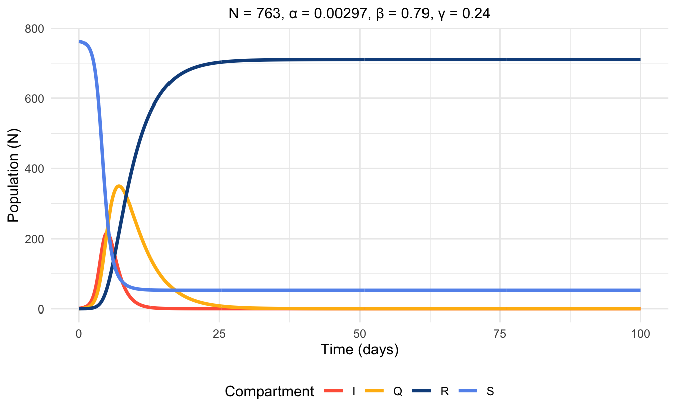
Figure 6.2: Time series plot of SIQR model at endemic equilibrium, simulated with parameter values.
6.2.4.1 Complex Models Vs. Parsimony in Real World Situations
As we have discussed, models may be too complex to fit the data. Key distinctions may be missing, which are vital to defining compartmental-specific data. In these scenarios, models are reduced to present a more general model while still being capable of great predictive power. In this specific scenario, the authors dive into attempting to use the SIQR model to use readily available data to define the perfect trends and relationships of COVID-19 in Missoula County, Montana, USA.
The authors state how the available data for one of the applied cases of the model included Active and New cases. However, an issue arose since the data values are not able to define \(\gamma\). This meant that individuals moved from Q to R were not defined, and thus, it was difficult to determine the transition number from individuals leaving the compartment. An individual might become recovered or quarantined but none of these outcomes are defined.
Because the data could not effectively be fit to the SIQR model, the author’s decided to reduce the model to an SIR model. In this situation, the Q and R compartments would be combined, resolving the issue of the unclear distinction between the two compartments. While this does remove the dynamics between quarantine and recovery, and removing the role that quarantine plays in the context, reducing to an SIR model is still the most effective choice. The SIR model allows for a powerful model to be utilized due to fewer parameters, preventing over fitting. While the SIQR model would have given more precise results with distinctions between the Q and R compartments, using an SIR model still allows for a general trend to be established about the spread of the disease in this certain population and case.
6.3 The SVIR Model
The model in this example is based on the parameters and variables defined in the articles by Ramponi et al. (2024) and Zhu X et al. (2024). [19] [29]
A non-specific disease that considers vaccination of the population is modelled. The model includes a “V” compartment for vaccinated individuals, and takes into account vaccination rate, vaccine effectiveness, and vaccine induced decline in the immune rate.
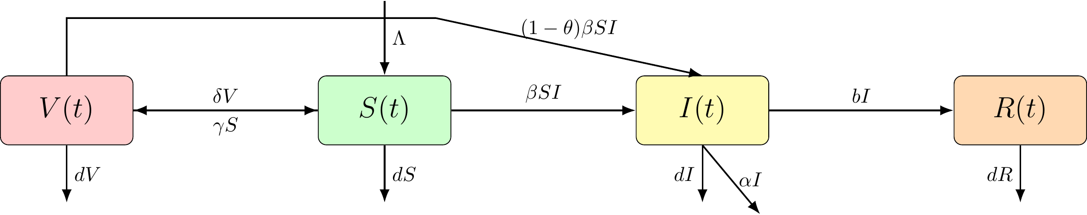
Figure 6.3: The VSIR compartmental model.
6.3.1 Defining the Parameters and Model Formulation
With \(N(t)\) representing the total population it can also be divided in to the four compartments: susceptible, vaccinated, infected and recovered.
Therefore, \(N(t) = V(t) + S(t) + I(t) + R(t)\)
The model assumes that after vaccination, people will develop immunity but after some time they will become susceptible again as the immunity wares off. Based on this, the following parameters can be defined:
\(\Lambda\) : susceptible individuals recruited by immigration/birth
\(\beta\) : effective contact rate between susceptible and infected individuals
\(d\) : natural death rate
\(\theta\) : vaccine effectiveness rate
\(\gamma\) : vaccination rate of susceptible individuals
\(b\) : cure rate of infected individuals
\(\alpha\) : disease induced mortality
\(\delta\) : loss rate of immunity
The epidemic dynamical model is given by the following four models :
\[ \begin{align*} \frac{dV}{dt} &= \gamma S -(1- \theta) \beta VI - (\gamma +d)V \\ \frac{dS}{dt} &= \Lambda + \delta V - \beta SI - (\gamma + d)S \\ \frac{dI}{dt} &= \beta SI + (1- \theta) \beta VI - (d+ \alpha + b)I \\ \frac{dR}{dt} &= bI - dR\\ \end{align*} \]
6.3.2 Defining the Disease Free Equilibrium
6.3.2.1 Solving for the Basic Reproduction Number
From here the basic reproduction number, \(R_0\), can be solved for using the next generation matrix method. When \(\theta = \gamma = \delta =0\), the system is then the SIR model essentially. Finding the regeneration and transfer matrix then gives:
\[ F_0 = \begin{bmatrix} \beta SI \\ 0 \\ 0 \end{bmatrix}, V_0 = \begin{bmatrix} (d+ \alpha + b) I \\ -bI + dR \\ - \Lambda + \beta SI +dS \end{bmatrix} \]
The next step would be to differentiate \(F_0\) and \(V_0\) and calculate the value of \(E_{00} = (S_{00},0,0) = (\frac{\Lambda}{d} , 0,0)\) which is at the DFE of the SIR model.
It can be found that
\[ F_0 = \begin{bmatrix} \beta S_{00} & 0 & 0 \\ 0 & 0 & 0 \\ 0 & 0 & 0 \end{bmatrix}, V_0 = \begin{bmatrix} (d + \alpha + b) & 0 & 0 \\ -b & d & 0 \\ \beta S_0 & 0 & d \end{bmatrix} \]
Since \(R_0 = \rho (F_0 V^{-1}_0)\),
\[ R_0 = \frac {\beta S_{00}}{d+b+\alpha } = \frac{\beta \Lambda}{d(d+b+ \alpha)} \]
Using this same process to solve for the SVIR. system’s disease free equlibrium, the derivatives can be set to 0, that is,
\(E_0 = (V_0, S_0, 0,0) = (\frac{\Lambda \gamma} {d (\delta + d +\gamma)} , \frac {\Lambda (\delta + d)} {d (\delta + d +\gamma)}, 0,0 )\)
Where \(x = (I, R, V, S)^T\), the regeneration matrix, \(F\) and the transfer matrix, \(V\) can be found to be :
\[ F = \begin{bmatrix} \beta SI + (1- \theta) \beta VI \\ 0\\ 0 \\ 0 \end{bmatrix}, V =\begin{bmatrix} (d + \alpha +b) I \\ -bI + dR\\ -\gamma S + (1-\theta) \beta VI +(\delta +d) V \\ - \Lambda - \delta V + \beta SI + (\gamma +d)S \end{bmatrix} \]
6.3.2.2 Computing the Basic Reproduction Number for the SVIR Model
To compute the basic reproduction number using the next-generation method, we separate the system into:
- new infection terms, denoted by \(\mathcal{F}\)
- all other transitions, denoted by \(\mathcal{V}\)
The system state is ordered as:
\[ x = (I, R, V, S)^T \]
From the SVIR model, only the infected class \(I\) receives new infections. Therefore, the new infection terms are:
\[ \mathcal{F} = \begin{bmatrix} \beta SI + (1-\theta)\beta V I\\ 0\\ 0\\ 0 \end{bmatrix} \]
All other terms in the system are collected into the transition matrix \(\mathcal{V}\):
\[ \mathcal{V} = \begin{bmatrix} (d + \alpha + b)I \\ -bI + dR\\ -\gamma S + (1-\theta)\beta V I + (\delta + d)V \\ -\Lambda - \delta V + \beta S I + (\gamma + d)S \end{bmatrix} \]
6.3.2.3 Linearization Around the Disease-Free Equilibrium
The disease-free equilibrium (DFE) for the SVIR model is:
\[ E_0 = (V_0, S_0, 0, 0) \]
where:
\[ V_0 = \frac{\Lambda\gamma}{d(\delta + d + \gamma)}, \quad S_0 = \frac{\Lambda(\delta + d)}{d(\delta + d + \gamma)} \]
We now compute the Jacobians \(D\mathcal{F}(E_0)\) and \(D\mathcal{V}(E_0)\).
6.3.2.4 Jacobian of \(\mathcal{F}\)
Only the first component of \(\mathcal{F}\) is non-zero:
\[ \mathcal{F}_1 = \beta SI + (1-\theta)\beta V I \]
Taking partial derivatives:
\[ \frac{\partial \mathcal{F}_1}{\partial I} = \beta S + (1-\theta)\beta V, \quad \frac{\partial \mathcal{F}_1}{\partial R} = 0 \]
Thus, the Jacobian evaluated at the DFE is:
\[ D\mathcal{F}(E_0)= \begin{bmatrix} \beta S_0 + (1-\theta)\beta V_0 & 0\\ 0 & 0 \end{bmatrix} \]
We denote this upper-left block as \(F\).
6.3.2.5 Jacobian of \(\mathcal{V}\)
The first two components of \(\mathcal{V}\) involve the infected subsystem:
\[ \mathcal{V}_1 = (d + \alpha + b)I, \quad \mathcal{V}_2 = -bI + dR \]
Taking partial derivatives:
\[ \frac{\partial \mathcal{V}_1}{\partial I} = d + \alpha + b, \quad \frac{\partial \mathcal{V}_2}{\partial I} = -b, \quad \frac{\partial \mathcal{V}_2}{\partial R} = d \]
Thus, the upper-left block of \(D\mathcal{V}(E_0)\) is:
\[ V = \begin{bmatrix} d + \alpha + b & 0\\ -b & d \end{bmatrix} \]
Lower blocks exist for the vaccinated and susceptible compartments, but they do not affect the computation of the reproduction number and are dropped.
6.3.3 Solving the SVIR Model
6.3.3.1 Forming the Next-Generation Matrix
The next-generation matrix is:
\[ FV^{-1} \]
First, compute the inverse of \(V\). For a matrix:
\[ \begin{bmatrix} a & 0\\ c & d \end{bmatrix} \]
the inverse is:
\[ \frac{1}{ad} \begin{bmatrix} d & 0\\ -c & a \end{bmatrix} \]
Applying this formula gives:
\[ V^{-1} = \frac{1}{d(d+\alpha + b)} \begin{bmatrix} d & 0\\ b & d+\alpha + b \end{bmatrix} \]
Now multiply:
\[ FV^{-1} = \begin{bmatrix} \frac{\beta\left(S_0 + (1-\theta)V_0\right)}{d+\alpha + b} & 0\\ 0 & 0 \end{bmatrix} \]
6.3.3.2 Computing the Reproduction Number
The basic reproduction number is the dominant eigenvalue (spectral radius) of \(FV^{-1}\):
\[ R_{\text{vac}} = \frac{\beta\left(S_0 + (1-\theta)V_0\right)}{d+\alpha + b} \]
Substituting the formulas for \(S_0\) and \(V_0\):
\[ S_0 = \frac{\Lambda(\delta + d)}{d(\delta + d + \gamma)}, \quad V_0 = \frac{\Lambda\gamma}{d(\delta + d + \gamma)} \]
6.3.3.3 Interpretation
- \(\dfrac{\beta}{d+\alpha+b}\) represents the expected number of
infections produced by an infectious individual before leaving the
infected class through recovery or death.
- \(S_0 + (1-\theta)V_0\) is the effective number of individuals at
risk, because:
- susceptible individuals contribute fully,
- vaccinated individuals contribute only by the fraction \((1-\theta)\) that the vaccine fails.
Thus:
- A higher vaccination rate \(\gamma\),
- a more effective vaccine \(\theta\),
both reduce \(R_{\text{vac}}\), helping to prevent the spread of infection.
6.3.4 Example with Parameter Values and Simulation
The following parameter values were retrieved from the article by Zhu et al. (2024) [29].
\(b= 0.0085\) (cure rate of infected individuals )
\(d = 0.005\) (natural death rate)
\(\theta = 0.6\) (vaccine effectiveness rate)
\(\beta = 0.29\) (effective contact rate between susceptible and infected individuals)
\(\delta = 0.005\) (loss rate of immunity)
\(\lambda = 10\) (susceptible individuals recruited by immigration/birth)
\(\alpha = 0.0099\) (disease induced mortality)
\(\gamma = 0.2\) (vaccination rate of susceptible individuals)
By plugging these parameter values into the previously solved equation for \(R_{vac}\), we obtain \(R_{vac} = 2.4716*10^4 \gg 1\) . Thus, we conclude that the endemic equilibrium is stable and the disease will persist.
Figure 6.4 represents a simulation based on these parameter values that displays the populations in each compartment of the VSIR model over the period of 1 year. Due to the set-up of the model, the time series plot does not follow the usual trends of compartmental model time series plots. In Figure 6.5, we focus on the initial 10 days of the VSIR simulation. From this, we can see that the compartments change very drastically within a single day (this looks like a vertical drop in the Vaccination compartment of Figure 6.4).
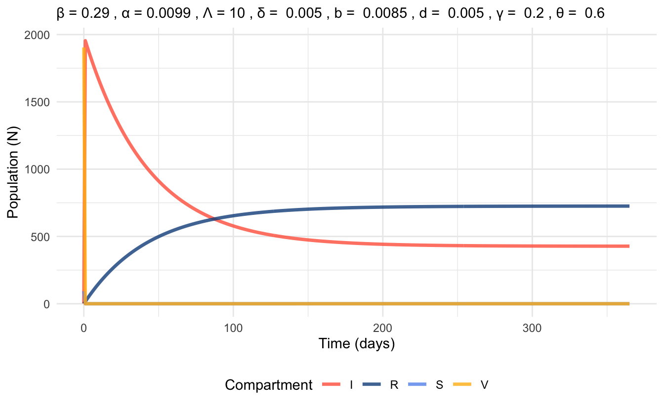
Figure 6.4: Time series plot of VSIR model at endemic equilibrium, simulated with parameter values for 1 year time scale.
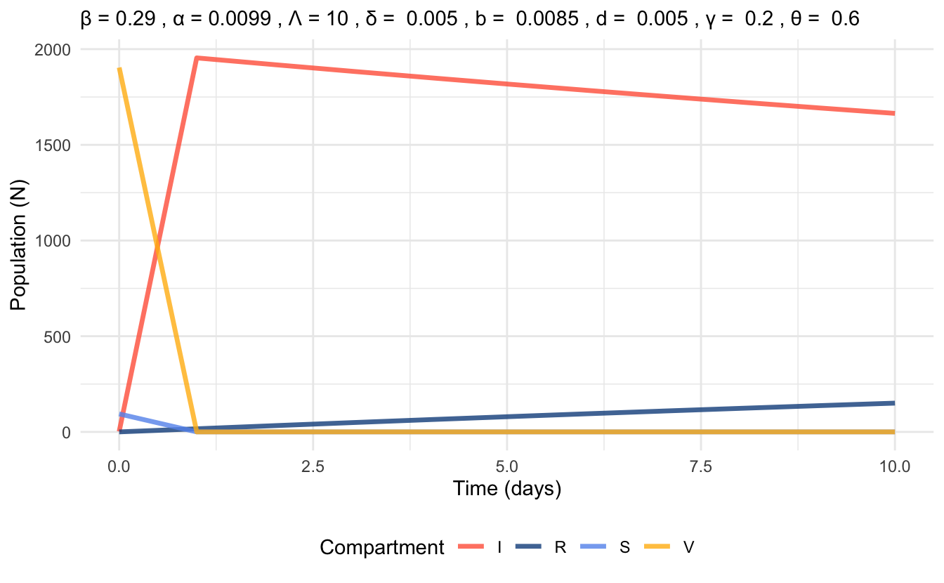
Figure 6.5: Time series plot of VSIR model at endemic equilibrium, simulated with parameter values for 10 days time scale.
6.4 The SAIR Model
SAIR model is a four compartment model that considers asymptomatic infected individuals (compartment “A”) as separate from the symptomatic individuals (compartment “I”).
In this section we will use the NGM to solve an example of SAIR that models COVID-19. This example was modified from a paper by Ouyang et al. (2025) [18], and it should be noted that the model includes parameters for vital dynamics (birth, death) and vaccination. This example showcases how models can become increasingly complex to solve and interpret when more parameters are involved.
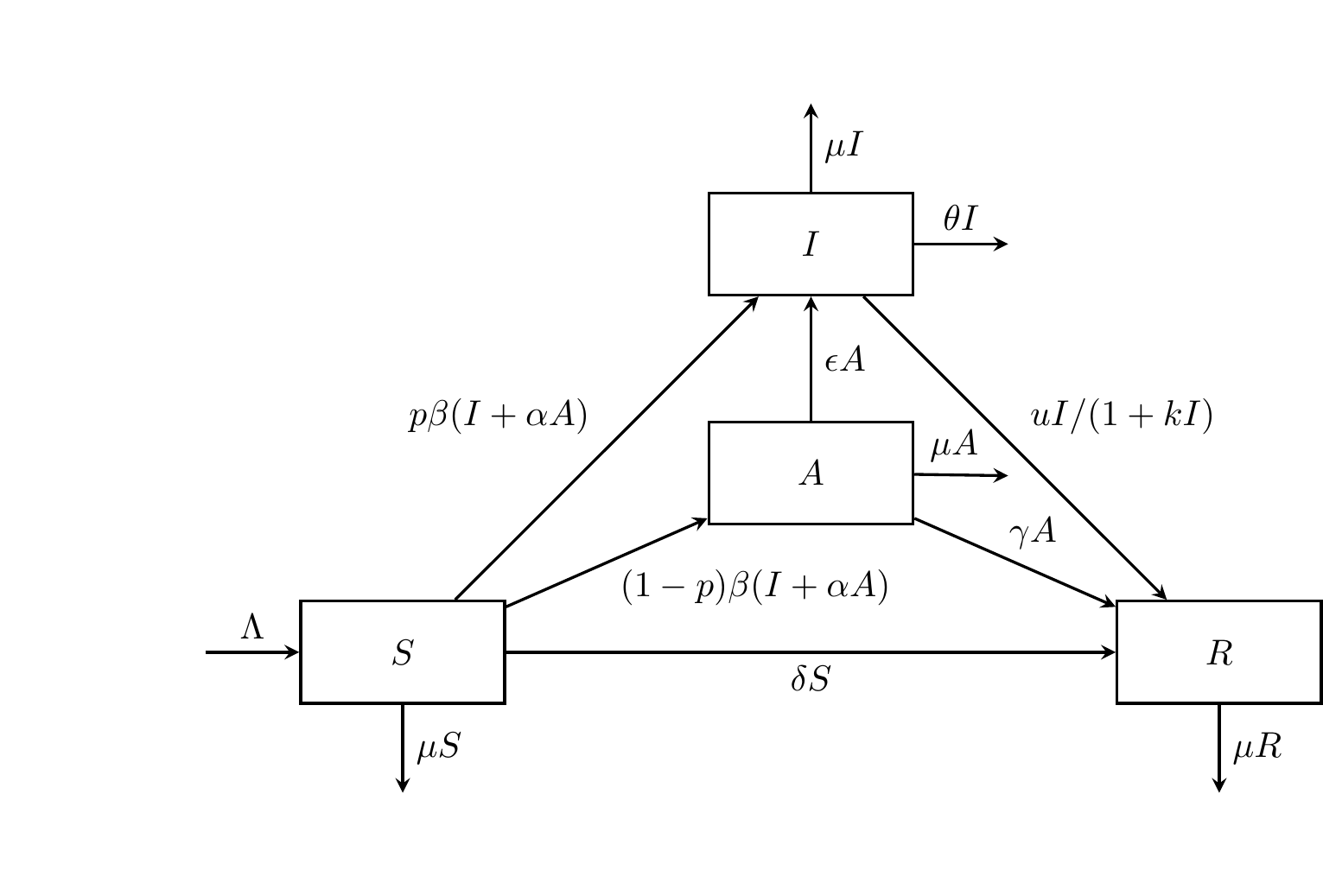
Figure 6.6: The SAIR compartmental model.
6.4.1 Defining the Parameters
SAIR Model Parameters:
\(p\): proportion of population that shows symptoms (\(0 < p < 1\))
- \((1-p)\): proportion of population that does not show symptoms
\(\beta(I+\alpha A)S\): new infection
\(\beta\): transmission rate
\(\alpha\): relative infectivity of asymptomatic infected (A) to symptomatic infected (I) (\(0 < a < 1\))
\(\gamma\): rate of the asymptomatic infected individuals’ self-healing (producing antibodies for resistance to diseases)
\(\epsilon\): rate of the asymptomatic infected individuals showing symptoms (if resistance to disease is poor)
\(\frac{uI}{1+kI}\): saturated treatment function represented by the Holling Type 2 Functional Response [20], which considers saturation of treatment rate when the numbers of infected are high.
- \(u\): cure rate of the infected individual
- \(k\): handling time
- \(\frac{u}{k}\): maximal treatment capacity, due to limited medical resources or handling time
\(\delta\): immunization rate of susceptible population from vaccination (this model considers vaccination without including a fifth compartment)
vital dynamics:
\(\Lambda\): recruitment rate of susceptible population (e.g. births, immigration)
\(\mu\): natural death rate per capita (all deaths unrelated to the disease)
\(\theta\): mortality rate of the disease (all deaths caused by the disease)
We define the differential equations for the SAIR Model as follows:
\[ \begin{align*} \ \dot{S} &= \Lambda -\beta(I+\alpha A)S - (\mu + \delta) S \\ \ \dot{A} &= (1-p)\beta(I+\alpha A)S-(\gamma + \epsilon + \mu)A \\ \ \dot{I} &= p\beta(I+\alpha A)S+\epsilon A - \frac{uI}{1+kI} - (\mu + \theta)I \\ \ \dot{R} &= \delta S + \frac{uI}{1+kI} + \gamma A - \mu R \\ \ \end{align*} \]
For the SAIR model, \(\dot{X} = \begin{bmatrix} \dot{A} \\ \dot{I}\\ \end{bmatrix}\), where X is the matrix representing the infected compartments.
6.4.2 Defining the Disease Free Equilibrium (DFE)
The Disease Free Equilibrium exists when all infected compartments (A and I), are set to 0. i.e. \(A=0\) and \(I=0\). (Definition 3.3).
\[ \begin{align*} \ \dot{S} &= \Lambda -\beta(I+\alpha A)S - (\mu + \delta) S &= 0 \\ \ \dot{A} &= (1-p)\beta(I+\alpha A)S-(\gamma + \epsilon + \mu)A &= 0 \\ \ \dot{I} &= p\beta(I+\alpha A)S+\epsilon A - \frac{uI}{1+kI} - (\mu + \theta)I &= 0 \\ \ \dot{R} &= \delta S + \frac{uI}{1+kI} + \gamma A - \mu R &= 0 \\ \ \end{align*} \]
By setting all of the differential equations to 0, we obtain that initial \(S\) is \(S = \frac{\Lambda}{\mu+\delta}\). Note that since we allow the population to vary by vital dynamics, we get \(N \neq 1\).
Therefore, at the DFE: \((S, A, I, R) = (\frac{\Lambda}{\mu+\delta}, 0, 0, \frac{\delta\Lambda}{\mu(\mu+\delta)})\)
6.4.3 Solving SAIR Model with NGM
We begin by finding \(R_0\), starting with the X matrix.
\[ \begin{align*} \ \dot{X} &= \begin{bmatrix} \dot{A} \\ \dot{I}\\ \end{bmatrix} \\ \ \dot{X} &= \begin{bmatrix} (1-p)\beta(I+\alpha A)S-(\gamma + \epsilon + \mu)A \\ p\beta(I+\alpha A)S+\epsilon A - \frac{uI}{1+kI} - (\mu + \theta)I \end{bmatrix} \\ \end{align*} \]
So then, from X we obtain: \(\boldsymbol{F} = \begin{bmatrix} (1-p)\beta(I+\alpha A)S \\ p\beta(I+\alpha A)S \end{bmatrix} = \begin{bmatrix} F_1 \\ F_2 \\ \end{bmatrix}\) and \(\boldsymbol{V} = \begin{bmatrix} (\gamma + \epsilon + \mu)A \\ -\epsilon A + \frac{uI}{1+kI} + (\mu + \theta)I \end{bmatrix} = \begin{bmatrix} V_1 \\ V_2 \\ \end{bmatrix}\)
Solving for the Jacobian matrices, we get:
\[ \begin{align*} \ \boldsymbol{F} &= J_F (x) = \begin{bmatrix} \frac{\partial F_1}{\partial A} & \frac{\partial F_1}{\partial I} \\ \frac{\partial F_2}{\partial A} & \frac{\partial F_2}{\partial I} \\ \end{bmatrix} = \begin{bmatrix} (1-p) \alpha \beta S & (1-p) \beta S \\ (p) \alpha \beta S & p \beta S \\\end{bmatrix} \\ \ \boldsymbol{V} &= J_V (x) = \begin{bmatrix} \frac{\partial V_1}{\partial A} & \frac{\partial V_1}{\partial I} \\ \frac{\partial V_2}{\partial A} & \frac{\partial V_2}{\partial I} \\ \end{bmatrix} = \begin{bmatrix} \gamma + \epsilon + \mu & 0 \\ -\epsilon & \frac{u}{(1+kI)^2} + \mu + \theta \\ \end{bmatrix} \\ \end{align*} \]
Since \(I = 0\): \[ \boldsymbol{V} = \begin{bmatrix} \gamma + \epsilon + \mu & 0 \\ -\epsilon & u + \mu + \theta \\ \end{bmatrix} \]
Then we can get: \[ \boldsymbol{V}^{-1} = \frac{1}{ (u + \mu + \theta) (\gamma + \epsilon + \mu)} \begin{bmatrix} u + \mu + \theta & 0 \\ \epsilon & \gamma + \epsilon + \mu \\ \end{bmatrix} \]
Next, recall that: \(NGM = \boldsymbol{F} \boldsymbol{V}^{-1}\)
\[ \begin{align*} \ \boldsymbol{F} \boldsymbol{V} ^{-1} &= \begin{bmatrix} (1-p) \alpha \beta S & (1-p) \beta S \\ (p) \alpha \beta S & p \beta S \\ \end{bmatrix} \frac{1}{ (u + \mu + \theta) (\gamma + \epsilon + \mu)} \begin{bmatrix} u + \mu + \theta & 0 \\ \epsilon & \gamma + \epsilon + \mu \\ \end{bmatrix} \\ \ &= \begin{bmatrix} (1-p) \alpha \beta S & (1-p) \beta S \\ (p) \alpha \beta S & p \beta S \\ \end{bmatrix} \begin{bmatrix} \frac{1}{\gamma + \epsilon + \mu} & 0 \\ \frac{\epsilon}{ (u + \mu + \theta) (\gamma + \epsilon + \mu)} & \frac{1}{u + \mu +\theta} \\ \end{bmatrix} \\ \ &= \begin{bmatrix} (\frac{1}{\gamma + \epsilon + \mu})(1-p) \alpha \beta S + (\frac{\epsilon}{ (u + \mu + \theta) (\gamma + \epsilon + \mu)}) (1-p) \beta S & (\frac{1}{u + \mu +\theta}) (1-p) \beta S \\ (\frac{1}{\gamma + \epsilon + \mu})p \alpha \beta S + (\frac{\epsilon}{ (u + \mu + \theta) (\gamma + \epsilon + \mu)}) p \beta S & (\frac{1}{u + \mu +\theta})p \beta S \\ \end{bmatrix} \\ \end{align*} \]
Use the formula \(det(J-\lambda I_n) = det(\lambda I_n -J) = 0\) to find the spectral radius, \(R_0\).
\[ \begin{align*} \ 0 &= det \left( \begin{bmatrix} (\frac{1}{\gamma + \epsilon + \mu})(1-p) \alpha \beta S + (\frac{\epsilon}{ (u + \mu + \theta) (\gamma + \epsilon + \mu)}) (1-p) \beta S & (\frac{1}{u + \mu +\theta}) (1-p) \beta S \\ (\frac{1}{\gamma + \epsilon + \mu})p \alpha \beta S + (\frac{\epsilon}{ (u + \mu + \theta) (\gamma + \epsilon + \mu)}) p \beta S & (\frac{1}{u + \mu +\theta})p \beta S \\ \end{bmatrix} -\lambda\begin{bmatrix} 1 & 0 \\ 0 & 1\end{bmatrix} \right) \\ \ 0 &= det \left( \begin{bmatrix} (\frac{1}{\gamma + \epsilon + \mu})(1-p) \alpha \beta S + (\frac{\epsilon}{ (u + \mu + \theta) (\gamma + \epsilon + \mu)}) (1-p) \beta S - \lambda & (\frac{1}{u + \mu +\theta}) (1-p) \beta S \\ (\frac{1}{\gamma + \epsilon + \mu})p \alpha \beta S + (\frac{\epsilon}{ (u + \mu + \theta) (\gamma + \epsilon + \mu)}) p \beta S & (\frac{1}{u + \mu +\theta})p \beta S - \lambda \\ \end{bmatrix} \right) \\ \ 0 &= \left( (\frac{1}{\gamma + \epsilon + \mu})(1-p) \alpha \beta S + (\frac{\epsilon}{ (u + \mu + \theta) (\gamma + \epsilon + \mu)}) (1-p) \beta S - \lambda \right) \left( (\frac{1}{u + \mu +\theta})p \beta S - \lambda \right) - \left( (\frac{1}{u + \mu +\theta}) (1-p) \beta S \right) \left( (\frac{1}{\gamma + \epsilon + \mu})p \alpha \beta S + (\frac{\epsilon}{ (u + \mu + \theta) (\gamma + \epsilon + \mu)}) p \beta S \right) \\ \end{align*} \]
Eventually, having substituted \(S = \frac{\Lambda}{\mu+\delta}\) into the equation, we obtain the following:
\[ R_0 = \frac{\beta \Lambda [(1-p)\alpha(u+\mu+\theta)+(1-p)\epsilon+p(\gamma+\epsilon+\mu)]}{(\mu+\delta)(\gamma+\epsilon+\mu)(u+\mu+\theta)} \]
We interpret this \(R_0\) as we have previously done: \(R_0 > 1\) indicates continuous spread of the disease (EE is stable), and \(R_0 < 1\) indicates that the disease will eventually die out (DFE is stable).
6.4.4 Example Parameters and Simulation
The following parameter values were retrieved from the article by Ouyang et al. (2025) [18], and also considers some demographic data from the United States of America in 2020.
\(p = 0.0065\) (proportion of symptomatic individuals)
\(\beta = 0.05\) (transmission rate)
\(\alpha = 0.00025\) (relative infectivity of asymptomatic individuals)
\(\gamma = 0.12\) (rate of asymptomatic self-healing)
\(\epsilon = 0.25\) (rate of asymptomatic individuals showing symptoms)
\(\delta = 0.04\) (immunization rate)
saturated treatment function:
\(u = 0.25\) (cure rate)
\(k = 20\) (handling time)
vital dynamics:
\(\Lambda = 1\) (recruitment rate)
\(\mu = 0.014\) (natural death rate)
\(theta = 0.01\) (COVID-19 death rate)
By plugging these parameter values into the previously solved equation for \(R_0\), we obtain \(R_0 = 2.208 > 1\). Thus, we conclude that the endemic equilibrium is stable and the disease will persist.
Figure 6.7 represents a simulation based on these parameter values that displays the populations in each compartment of the SAIR model over the period of 2 years.
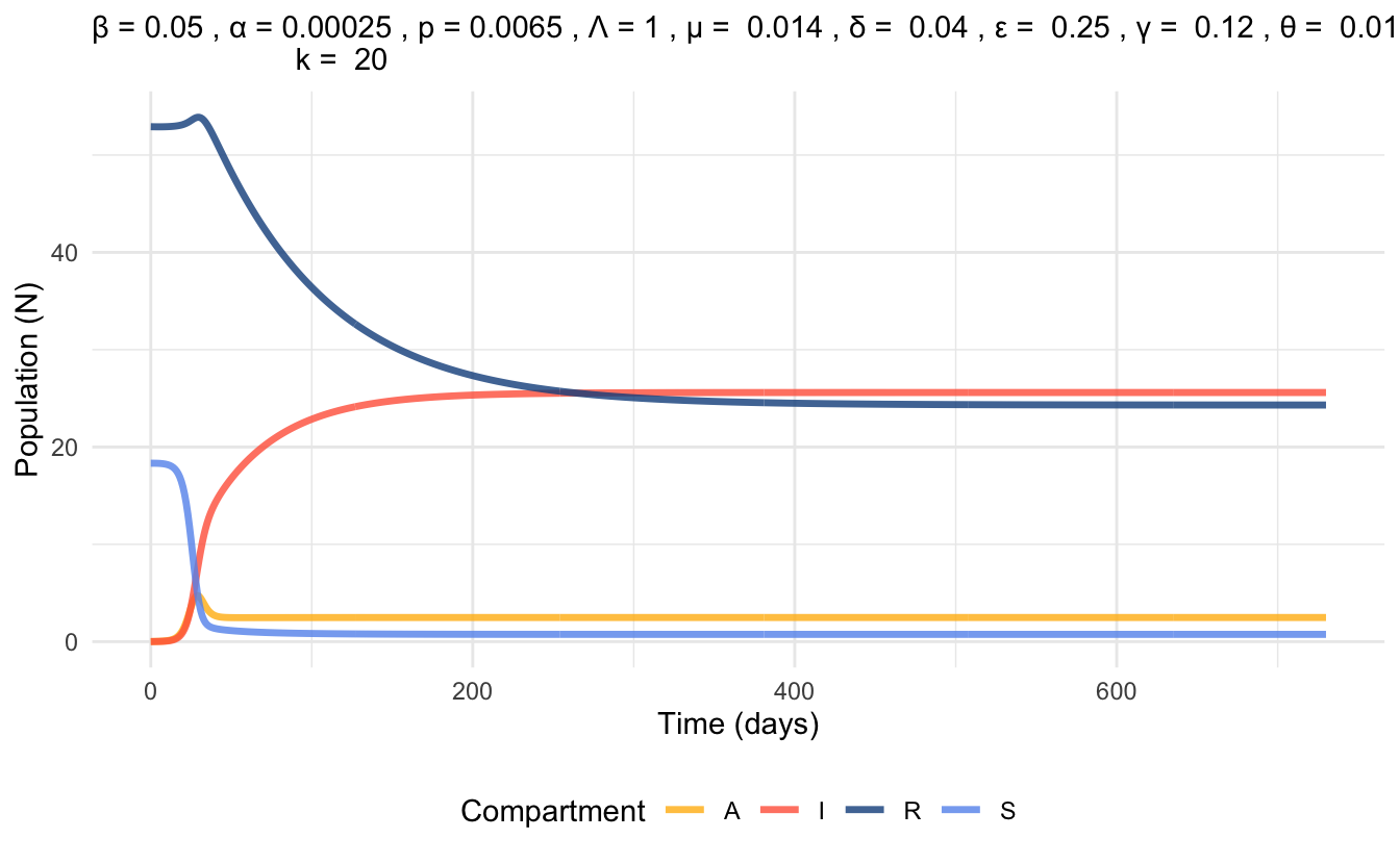
Figure 6.7: Time series plot of SAIR model at endemic equilibrium, simulated with parameter values.